Topics and concepts covered in the first 5 weeks of ECE538 at Purdue University.

Week 1: DT Signals and Systems Basics

The purpose of this week was to easily slide into the course material and work with convolution in the discrete time case.

Sampling (basics)

Sampling is the process of converting a continuous time signal into a discrete time signal. The sampling done in this course is all even-width sampling, which means

$$x[n]\overset{\Delta}{=}x(nT_s) \forall n \in \mathbb{Z}$$

Where $T_s$ is called the sampling period, with a corresponding $f_s = \frac{1}{T_s}$ as the sampling frequency.

Special Signals

Common signals to work with are:

Unit step:

$$ u[n-n_0] = \begin{cases} 0 & n < n_0 \\ 1 & n\geq n_0 \\ \end{cases} $$

DT Impulse:

$$ \delta[n-n_0] = \begin{cases} 0 & n \neq n_0 \\ 1 & n = n_0 \\ \end{cases} $$$$e^{j(\omega_0 + 2\pi k)n}=e^{j\omega_0 n}$$

2. Periodicity:

2a. Condition on Periodicity

$$e^{j\omega_0(n+N)}=e^{j\omega_0 n} \iff \frac{\omega_0}{2\pi} \in \mathbb{Q}$$

2b. Fundamental Period: find the smallest k so that

$$N_0 = k\frac{2\pi}{\omega_0} \in \mathbb{Z}$$

Convolution

Convolution in discrete time is defined as

$$x[n]*h[n]=\sum_{k=-\infty}^{\infty}x[k]h[n-k]=\sum_{k=-\infty}^{\infty}h[k]x[n-k]$$

LTI systems operate on the input by convolution of the impulse response. This can be shown with the below approach:

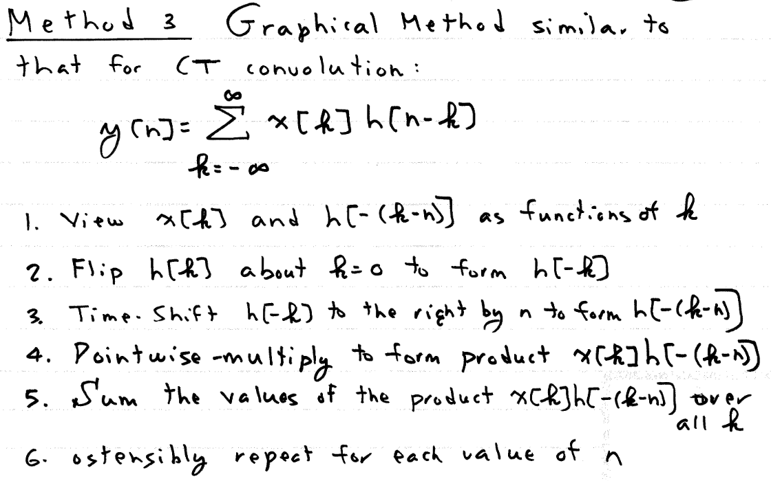
$$y[n]=T\{x[n]\}=T\{\sum_{k=-\infty}^{\infty}x[k]\delta[n-k]\}=\sum_{k=-\infty}^{\infty}x[k]T\{\delta[n-k]\}=\sum_{k=-\infty}^{\infty}x[k]h[n-k]=x[n]*h[n]$$

Methods of Convolution

1. Directly apply the formula
2. Graphical convolution

Properties of Convolution

1. Associative
2. Commutative
3. Distributive

Week 2: Autocorrelation and Cross-Correlation

This is where new content for the course starts. The purpose of this week was to understand autocorrelation, its properties, and its applicatiions.

The idea of autocorrelation is to see if a particular signal is embedded in a received signal. This is often used in radar applications, where the received signal is a time-delayed version of the original transmitted signal, with some noise added. Take the below example:

$$y[n]=\sum_{k=-\infty}^{\infty}a_kx[n-Dk]+w[n]$$

Notice the following:

$$z[n]=y[n]*x^*[-n]=\sum_{k=-\infty}^{\infty}a_kx[n-Dk]*x^*[-n]+w[n]*x^*[-n]$$$$z[n]=\sum_{k=-\infty}^{\infty}a_kx[n]*\delta(n-Dk)*x^*[-n]+w[n]*x^*[-n]$$$$z[n]=\sum_{k=-\infty}^{\infty}a_kx[n]*x^*[-n]*\delta(n-Dk)+w[n]*x^*[-n]$$$$z[n]=\sum_{k=-\infty}^{\infty}a_kr_{xx}[n]*\delta(n-Dk)+w[n]*x^*[-n]$$

Now, we define cross-correlation:

$$r_{xy}[l]=x[l]*y^*[-l]=\sum_{k=-\infty}^{\infty}x[k]y^*[k-l]$$

Autocorrelation occurs when $y=x$:

$$r_{xx}[l]=x[l]*x^*[-l]=\sum_{k=-\infty}^{\infty}x[k]x^*[k-l]$$

Thus,

$$z[n]=\sum_{k=-\infty}^{\infty}a_kr_{xx}[n-Dk]+r_{wx}$$

With the appropriate choice of $x[n]$, $r_{xx}[n-Dk]=\delta[n-Dk]$, giving a clear signal that indicates when $x[n-Dk]$ was received.

Properties of Autocorrelation / Useful TidBits

1. Hemertian Symmetry: $$r_{xx}[-n]=r_{xx}^*[n]$$ $$r_{xx}[n]=r_{xx}^*[-n]$$ Proof: $$r_{xx}[-n]=x[-n]*x^*[n]=x^*[n]*x[-n]$$ $$r_{xx}^*[n]=x^*[n]*x[-n]$$
2. Zero property: $$|r_{xx}[n]|\leq |r_{xx}[0]| \forall n$$
3. DTFT: $$\sum_{k=-\infty}^{\infty}r_{xx}[n]e^{-j\omega n} \geq 0, \in \mathbb{R}, \forall \omega$$
4. Time Invariance: $$x[n]*x^*[-n]=x[n]*x^*[-n]|_{n=n-n_0}$$
5. Frequency Shift: $$y[n]=e^{j(\omega_0 n + \theta_0)}x[n]\Rightarrow r_{yy}[n]=e^{j\omega_0 n}r_{xx}[n]$$
6. LTI Systems: $$y[n] = x[n]*h[n] \Rightarrow r_{yy}[n]=r_{xx}[n] * r_{hh}[n]$$
7. Geometric Autocorrelation: $$x[n] = a^nu[n] \Rightarrow r_{xx}[n]=\frac{1}{1-a^2}a^{|n|}, |a|<1$$
8. Autocorrelation in the Frequency Domain (see properties 3 and 4 in the Z-transform properties section): $$r_{xx}[n]=x[n]*x^*[-n]\Rightarrow S_{xx}(e^{j\omega})=X(e^{j\omega})X^*(e^{j\omega})=|X(e^{j\omega})|^2$$

Week 3: Z-Transform & DT Fourier Transform

The purpose of this week is to revisit the idea of the Z-transform and DTFT.

Derivation / Motivation

Z-Transform

As stated previously, the geometric series is the eigenfunction for LTI systems in discrete time:

$$y[n]=h[n]*x[n]=\sum_{k=-\infty}^{\infty}h[k]a^{n-k}=(\sum_{k=-\infty}^{\infty}h[k]a^{-k})a^n=H(a)a^n$$

Thus, we define

$$H(z)=Z\{h[n]\}=\sum_{n=-\infty}^{\infty}h[n]z^{-n}$$

DTFT

Let $x[n]=e^{j\omega_0 n}$ and pass into LTI system:

$$y[n]=h[n]*x[n]=\sum_{k=-\infty}^{\infty}h[k]e^{j\omega_0(n-k)}=(\sum_{k=-\infty}^{\infty}h[k]e^{-j\omega k})e^{j\omega_0 n}=H(e^{j\omega_0})e^{j\omega_0 n}$$

Thus, the DTFT is nothing but evaluating the Z-transform on the unit circle:

$$H(e^{j\omega})=DTFT\{h[n]\}=H(z)|_{z=e^{j\omega}}=\sum_{n=-\infty}^{\infty}h[n]e^{-j\omega_0 n}$$

Stability

First, express $H(z)$ in terms of poles and zeroes (a relatively unrestrictive assumption, see Difference Equations):

$$H(z)=\frac{\Pi_{k=0}^{M}(z-z_k)}{\Pi_{k=0}^{N}(p-p_k)}$$

Notice first that the radius of convergence of $H(z)$ must be given by $|z|>|p_{max}|$, where $p_{max}$ is the pole with the largest magnitude.

Notice second that the definition of the Z-transform and the triangle inequality obtains:

$$|H(z)|\leq \sum_{n=-\infty}^{\infty}|h[n]z^{-n}|$$

We know that BIBO stability requires $$$\sum_{n=-\infty}^{\infty}|h[n]| < \infty$

So evaluate the above at $z=e^{j\omega}$

$$|H(e^{j\omega})|\leq \sum_{n=-\infty}^{\infty}|h[n]|<\infty$$

This means that the radius of convergence must include the unit circle. Since $|z_{max}|=1>|p_{max}|$, this means that in order for a system to be BIBO stable, all poles must be within the unit circle.

Difference Equations

A difference equation is the DT analogy to a CT differential equation. They are given in the below form:

$$y[n]=\sum_{k=0}^{M}a_kx[n-k]-\sum_{k=1}^{N}b_ky[n-k]$$

Simple Analysis

Taking the Z-transform of both sides:

$$Y(z)=\sum_{k=0}^{M}a_kX(z)z^{-k}-\sum_{k=1}^{N}b_kY(z)z^{-k}$$

Solving for $H(z)=\frac{Y(z)}{X(z)}$:

$$H(z)=\frac{\sum_{k=0}^{M}a_kz^{-k}}{1+\sum_{k=1}^{N}b_kz^{-k}}$$

From here, pole-zero analysis can be performed.

FIR, IIR

Finite impulse response (FIR) systems often take the following form:

$$y[n]=\sum_{k=0}^{M}a_kx[n-k]$$

As can be seen:

$$h[n]=\sum_{k=0}^{M}a_k\delta[n-k]$$

.

$\fbox{The defining characteristic of FIR systems is that they have no (nonzero) poles, only zeros.}$

Infinite impulse response (IIR) systems take the form of a general difference equation. $\fbox{If a system has a nonzero pole, it is IIR.}$

The names of both types come from the length of time it takes for the impulse response to stay at 0. This never happens for IIRs, and always happens for FIRs.

Pole-Zero Analysis

It is useful to be able to look at just $|H(z)|$ or $\angle H(z)$ for any given $z$. Since $H(z)$ can usually be written as a rational function of polynomials, this analysis is not difficult if we understand complex numbers.

$$H(z)=\frac{\Pi_{k=0}^{M}(z-z_k)}{\Pi_{k=0}^{N}(p-p_k)}$$$$|H(z)|=\frac{\Pi_{k=0}^{M}|z-z_k|}{\Pi_{k=0}^{N}|p-p_k|}$$

$$\angle H(z)=\Pi_{k=0}^{M}\angle(z-z_k)-\Pi_{k=0}^{N}\angle(p-p_k)$$

This can be easily programmed and calculated.

Properties / Useful TidBits

1. Time shifting $$Z\{x[n-n_0]\}=z^{-n_0}X(z)$$
2. Convolution $$Z\{x[n]*h[n]\}=X(z)H(z)$$
3. Conjugation $$Z\{x^*[n]\}=X^*(z^*)$$
4. Time-Reversal $$Z\{x[-n]\}=X(\frac{1}{z})$$
5. Geometric Sequence $$Z\{a^nu[n]\}=\frac{z}{z-a} \forall |z|>|a|$$
6. Derivative in Z-domain $$Z\{nx[n]\}=-z\frac{d}{dz}X(z)$$
7. Domain Stretch in Z-domain $$Z\{a^nx[n]\}=X(\frac{z}{a})$$

Week 4: Frequency Response of LTI Systems

The purpose of this week was to understand how pole/zero placement of the impulse response can affect the frequency response of an LTI system.

All-Pass Filter

Basic Analysis

All-pass filters have the below impulse response:

$$H(e^{j\omega})=G\frac{e^{j\omega}-\frac{1}{p^*}}{e^{j\omega}-p}$$

Proof:

$$G\frac{e^{j\omega}-\frac{1}{p^*}}{e^{j\omega}-p}=G\frac{-\frac{e^{j\omega}}{p^*}(e^{-j\omega}-p^*)}{e^{j\omega}-p}=G\frac{-\frac{e^{j\omega}}{p^*}(e^{j\omega}-p)^*}{e^{j\omega}-p}$$

Therefore

$$|H(e^{j\omega})|=|G|\frac{|-\frac{e^{j\omega}}{p^*}||(e^{j\omega}-p)^*|}{|e^{j\omega}-p|}=\frac{|G|}{|p|}, \forall \omega$$

Which is an all-pass filter. Notice that $|G|=|p|$ normalizes the all-pass.

Connection to Autocorrelation

Recall that

$$DTFT\{r_{hh}[n]\}=|H(e^{j\omega})|^2=(\frac{|G|}{|p|})^2$$

Therefore

$$h[n]*h^*[-n]=(\frac{|G|}{|p|})^2\delta[n]$$

Time-Domain

$$H(z)=p\frac{z-\frac{1}{p^*}}{z-p}=p\frac{z}{z-p}-\frac{p}{p^*}z^{-1}\frac{z}{z-p}$$

Thus

$$h[n]=pp^nu[n]-e^{j2\angle p}p^{n-1}u[n-1]$$

A more common expression can be obtained with further manipulation:

$$=p\delta[n]+pp^nu[n-1]-\frac{e^{j2\angle p}}{p}p^nu[n-1]=p\delta[n]+(p-\frac{e^{j2\angle p}}{p})p^nu[n-1]=p\delta[n]+(p-\frac{e^{j2\angle p}}{p})p^{n}u[n] - (p-\frac{e^{j2\angle p}}{p})\delta[n]=\frac{e^{j2\angle p}}{p}\delta[n]+(\frac{p^2-e^{j2\angle p}}{p})p^{n}u[n]$$

Obtaining

$$h[n]=\frac{1}{p}(e^{j2\angle p}\delta[n]+(p^2-e^{j2\angle p})p^{n}u[n])$$

Notice that if $p \in \mathbb{R}$

$$\boxed{h[n]=\frac{1}{p}(\delta[n]+(p^2-1)p^{n}u[n])}$$

Notch Filter

Nothced filters have the following impulse response:

$$H(e^{j\omega})=G\frac{\Pi_{k=0}^{M}(e^{j\omega}-e^{j\omega_{k}})}{\Pi_{k=0}^{M}(e^{j\omega}-re^{j\omega_{k}})}$$

The key is that the zeros lie on the unit circle at the frequencies that are notched out. The poles create a contrast between the surrounding frequencies and the notched frequencies. The closer the poles are to the unit circle, the narrower the notching is.

Notch Filter and All-Pass Filter Connection

Two All-Pass filters in parallel can create a notch filter. Observe the following:

$$H_1(z)=\frac{z-\frac{1}{p^*}}{z-p}$$

$$H_2(z)=\frac{z+\frac{1}{p^*}}{z+p}$$

Notice that the above filters have passband gain of $\frac{1}{|p|}$

$$H_1(z)+H_2(z)=\frac{z-\frac{1}{p^*}}{z-p}+\frac{z+\frac{1}{p^*}}{z+p}=\frac{(z-\frac{1}{p^*})(z+p)+(z+\frac{1}{p^*})(z-p)}{(z-p)(z+p)}$$

$$\frac{(z-\frac{1}{p^*})(z+p)+(z+\frac{1}{p^*})(z-p)}{(z-p)(z+p)}=\frac{z^2+z(p-\frac{1}{p^*})-\frac{p}{p^*}+z^2-z(p-\frac{1}{p^*})-\frac{p}{p^*}}{(z-p)(z+p)}=2\frac{z^2-\frac{p}{p^*}}{(z-p)(z+p)}=2\frac{(z+\sqrt{\frac{p}{p^*}})(z-\sqrt{\frac{p}{p^*}})}{(z-p)(z+p)}$$

Finally, we obtain

$$H_1(z)+H_2(z)=2\frac{(z-e^{j(\angle p+\pi)})(z-e^{j\angle p})}{(z-p)(z+p)}$$

Which is a notch filter with notching frequencies $\omega = \{\angle p, \angle p + \pi\}$

Pole-Zero Cancellation: Difference Equations

Consider the following system:

$$y[n]=e^{j2\pi\frac{l}{n}}y[n-1]+x[n]-x[n-N]$$

With $l < N$

Basic Analysis

This system fits the form of IIR, but in fact is FIR.

$$H(z)=\frac{1-z^{-N}}{1-e^{j2\pi\frac{l}{n}}z^{-1}}=\frac{z^{N}-1}{z^{N}-e^{j2\pi\frac{l}{n}}z^{N-1}}=\frac{\Pi_{k=0}^{N-1}(z-e^{j\frac{2\pi k}{N}})}{z^{N-1}(z-e^{j2\pi\frac{l}{n}})}=\frac{\Pi_{k=0}^{l-1}(z-e^{j\frac{2\pi k}{N}})\Pi_{k=l+1}^{N-1}(z-e^{j\frac{2\pi k}{N}})}{z^{N-1}}$$

As can be seen, the impulse response simply consists of zeros, without any (nonzero) poles, because a pole/zero cancellation occured.

Frequency Response

We revert to the stage before the pole-zero cancellation, to make our work easier:

$$H(e^{j\omega})=\frac{e^{j\omega N}-1}{e^{j\omega (N-1)}(e^{j\omega}-e^{j2\pi\frac{l}{n}})}$$

And make use of the “half-angle trick”:

$$ H(e^{j\omega})=\frac{(e^{j\omega \frac{N}{2}}-e^{-j\omega \frac{N}{2}})e^{j\omega \frac{N}{2}}}{(e^{j\frac{\omega}{2}}e^{-j\pi\frac{l}{n}}-e^{-j\frac{\omega}{2}}e^{j\pi\frac{l}{n}})e^{j\frac{\omega}{2}}e^{j\pi\frac{l}{n}}e^{j\omega (N-1)}} =\frac{(e^{j\omega \frac{N}{2}}-e^{-j\omega \frac{N}{2}})e^{j\omega \frac{N}{2}}}{(e^{j(\frac{\omega}{2}-\pi\frac{l}{n})}-e^{-j(\frac{\omega}{2}-\pi\frac{l}{n})})e^{j(\frac{\omega}{2}+\pi\frac{l}{n}+\omega (N-1))}} = \frac{(e^{j\omega \frac{N}{2}}-e^{-j\omega \frac{N}{2}})e^{j(\omega \frac{1-N}{2}-\pi\frac{l}{n})}}{(e^{j(\frac{\omega}{2}-\pi\frac{l}{n})}-e^{-j(\frac{\omega}{2}-\pi\frac{l}{n})})} $$