ECE538 Week 1: Discrete Time Signals and Systems Basics
The purpose of this week was to easily slide into the course material and work with convolution in the discrete time case.
Sampling (basics)
Sampling is the process of converting a continuous time signal into a discrete time signal. The sampling done in this course is all even-width sampling, which means
$$x[n]\overset{\Delta}{=}x(nT_s) \forall n \in \mathbb{Z}$$Where $T_s$ is called the sampling period, with a corresponding $f_s = \frac{1}{T_s}$ as the sampling frequency.
Special Signals
Common signals to work with are:
Unit step:
$$ u[n-n_0] = \begin{cases} 0 & n < n_0 \\ 1 & n\geq n_0 \\ \end{cases} $$DT Impulse:
$$ \delta[n-n_0] = \begin{cases} 0 & n \neq n_0 \\ 1 & n = n_0 \\ \end{cases} $$Geometric:
$x(t)=e^{-\frac{t}{\tau}}u(t)$ is the eigenfunction of all LTI systems. This makes it a very important function in continuous time systems.
The geometric sequence is the equivalent of the exponential function in discrete time systems.
$$x[n]=x(nT_s)=e^{-\frac{nT_s}{\tau}}u(nT_s)=(e^{-\frac{T_s}{\tau}})^{n}u[n]=a^nu[n]$$$$x[n]=a^nu[n]$$DT Sine Wave:
$$x[n]=e^{j\omega_0 n}$$Properties:
- Aliasing $$e^{j(\omega_0 + 2\pi k)n}=e^{j\omega_0 n}$$
- Periodicity:
2a. Condition on Periodicity
$$e^{j\omega_0(n+N)}=e^{j\omega_0 n} \iff \frac{\omega_0}{2\pi} \in \mathbb{Q}$$2b. Fundamental Period: find the smallest k so that
$$N_0 = k\frac{2\pi}{\omega_0} \in \mathbb{Z}$$Convolution
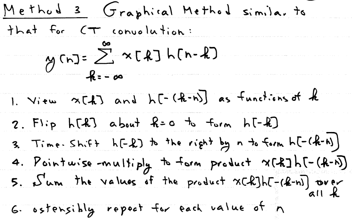
Convolution in discrete time is defined as
$$x[n]*h[n]=\sum_{k=-\infty}^{\infty}x[k]h[n-k]=\sum_{k=-\infty}^{\infty}h[k]x[n-k]$$LTI systems operate on the input by convolution of the impulse response. This can be shown with the below approach:
$$y[n]=T\{x[n]\}=T\{\sum_{k=-\infty}^{\infty}x[k]\delta[n-k]\}=\sum_{k=-\infty}^{\infty}x[k]T\{\delta[n-k]\}=\sum_{k=-\infty}^{\infty}x[k]h[n-k]=x[n]*h[n]$$Methods of Convolution
- Directly apply the formula
- Graphical convolution
Properties of Convolution
- Associative
- Commutative
- Distributive