The purpose of this week is to derive the relationship between the CTFT and DTFT, thus dipping our toes into sampling theory.

$$\boxed{X_s(\omega F_s) = X(\omega)}$$

1. CTFT, DTFT Relationship

1.1 Prerequisites

First, we shall establish some variables and concepts.

Let $x_a(t)$ be the analog signal to be sampled into $x[n]$ by $x_s(t)$ with a sampling frequency $F_s=\frac{1}{T_s}$. The relationships between these variables are:

$$x[n]=x_a(nT_s)$$

$$x_s(t)=x_a(t)\sum_{n=-\infty}^{\infty}\delta(t-nT_s)$$

DTFT:

$$X(\omega)=\sum_{n=-\infty}^{\infty}x[n]e^{-j\omega n}$$

CTFT:

$$X_a(\omega)=\int_{t=-\infty}^{\infty}x_a(t)e^{-j\omega t}dt$$

The relationship between $x_s(t)$ and $x[n]$ is the central topic we’d like to discuss.

1.2 Derivation

First, notice the following:

$$x_s(t)=x_a(t)\sum_{n=-\infty}^{\infty}\delta(t-nT_s) \Rightarrow X_s(\omega) = X_a(\omega)*F_s\sum_{n=-\infty}^{\infty}\delta(\omega-2\pi nF_s)$$

$$X_s(\omega) = F_s\sum_{n=-\infty}^{\infty}X_a(\omega-2\pi nF_s)$$

Hold this in your pocket, we now move on. From the following:

$$x_s(t)=x_a(t)\sum_{n=-\infty}^{\infty}\delta(t-nT_s)=\sum_{n=-\infty}^{\infty}x_a(nT_s)\delta(t-nT_s)$$

$$X_s(\omega) = \sum_{n=-\infty}^{\infty}x_a(nT_s)e^{-j\omega nT_s}=\sum_{n=-\infty}^{\infty}x[n]e^{-j\omega nT_s}$$

Now perform the following substitution:

$$\boxed{X_s(\omega F_s) = \sum_{n=-\infty}^{\infty}x[n]e^{-j\omega n F_sT_s}=\sum_{n=-\infty}^{\infty}x[n]e^{-j\omega n}=X(\omega)}$$

1.3 Interpretation

To interpret this result, notice that the input to $X_s(\omega)$ can be called the analog frequency, $\omega_a$ and the input to $X(\omega)$ can be called the digital frequency, $\omega_d$. Therefore, we have

$$\omega_a=\omega_d F_s$$

Another note of importance is that $X_s(\omega F_s) = X(\omega)$, combined with the fact that

$$X_s(\omega) = F_s\sum_{n=-\infty}^{\infty}X_a(\omega-2\pi nF_s)$$

Means

$$X(\omega) = F_s\sum_{n=-\infty}^{\infty}X_a(\omega F_s-2\pi nF_s)=F_s\sum_{n=-\infty}^{\infty}X_a(F_s(\omega -2\pi n))$$

Which means that the DTFT takes the analog spectrum and compressed it by $F_s$, then repeats it at every mutliple of $2\pi$ and adds the result. Notice that this explains aliasing - if $F_s$ is too small, the compression does not prevent overlapping of neighboring spectra.

2. Ideal Reconstruction, or D2A Conversion

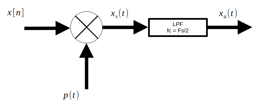
In order to reconstruct $x_a(t)$ from $x[n]$, we use $x_s(t)$:

$$x_s(t) = \sum_{n=-\infty}^{\infty}x[n]\delta(t-nT_s)$$$$X_s(f) = F_s\sum_{n=-\infty}^{\infty}X_a(f- nF_s)$$

As can be seen, if you pass $x_s(t)$ into a low pass filter, then you can retrieve $x_a(t)$.