The purpose of this week is to finish up reconstruction and introduce upsampling.

1. Reconstruction (D2A Conversion)

The below figure represents the D2A conversion process in blocks. We first focus on the LPF, then the upsampler.

1.1 Ideal Reconstruction Filters

Recall that we have

$$X_s(f) = F_s\sum_{n=-\infty}^{\infty}X_a(f- nF_s)$$

And thus a LPF centered around the first copy of $X_a(f)$ is used to recover $x_a(t)$.

The first LPF to consider is a simple rectangle. However, notice that the time domain signal required for this rectangle is an infinite-length sinc wave. Major distortion in the form of Gibb’s phenomenon is present when truncating the signal for practical applications, thus we search for better alternatives.

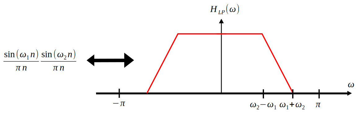
The next LPF to consider is inspired by the first - by moving from $sinc(t)$ to $sinc^2(t)$. Consider that $sinc^2(t)$ has a more signal power concentrated near the center of the wave than simple $sinc(t)$ does, therefore this seems promising. However, remember that $sinc^2(t)$ gives a triangle in the frequency domain, which does not preserve the property that the baseband $X_a(f)$ is preserved after the filter. Therefore, the below solution is chosen - by convolving two rectangles of different widths, we achieve the desired result.

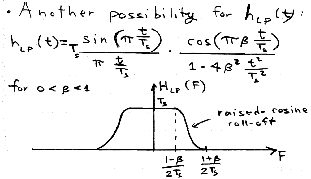
The final LPF to consider is the raised cosine filter. This also has the desired properties for reconstruction.

1.2 Use of Upsampling in Reconstruction

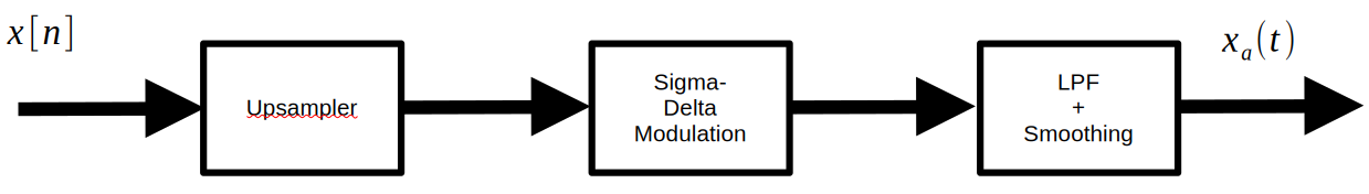
In order to understand why upsampling is used in the reconstruction process, we must first understand the sigma-delta modulator. In short, sigma-delta modulation is an efficienct scheme for A2D and D2A conversion that changes its output level only one quantization level at a time by comparing the current value to the desired value and updating accordingly. The below figure illustrates this behavior - initially, the SDM output is 0, but it climbs at each step until it reaches the steady state of the analog signal.

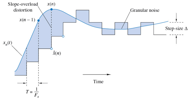
Upsampling is used before this process because SDM is a much more accurate process the quicker you sample. So, if we can somehow digitally change the sampling frequency, we can make D2A a much more accurate process.

2. Upsampling

The goal of digital upsampling is to acquire $x_a(\frac{nT_s}{L})$ from our samples of $x_a(nT_s)$ only. For now, let $L$ be an integer.

In short, we desire a digital system with relation

$$y[n] = x[\frac{n}{L}] = \sum_{k=-\infty}^{\infty}x[k]\delta[n-kL]$$

Notice that in the frequency domain, the relation is

$$Y(\omega)=X(L\omega)$$

This is useful in digital subbanding

2.1 Inefficient Method - Zero Inserts

Recall that through the process of reconstruction, we obtain:

$$x_a(t)=[\sum_{k=-\infty}^{\infty}x[k]\delta(t-kT_s)]*h_{LP}(t)$$

We wish to obtain

$$y[n]=x_a(\frac{nTs}{L})=[\sum_{k=-\infty}^{\infty}x[k]\delta[\frac{n}{L}-k]]*h_{LP}[\frac{n}{L}]$$

Which amounts to

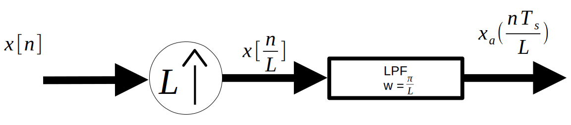
$$y[n]=x_a(\frac{nTs}{L})=x[\frac{n}{L}]*h_{LP}[\frac{n}{L}]$$

This is schematically represented in the below figure.

The $x[\frac{n}{L}]$ term is represented by the circle with an L inside of it. This element inserts $L-1$ zeros in between each sample of $x[n]$. Thus, the function of the LPF can be seen as “filling in” those zeros through convolution.

However, this means that this process is incredibly inefficienct, as most of the convolution performed when passing the zero-insert output into the LPF is just multiplication by 0. We hunt for a more efficient version in the rest of this chapter.

2.2 Efficient Method - Fractional Time Shift Filters

First, notice that $y[n]$ can be written as below:

$$y[n]=\sum_{k=-\infty}^{\infty}x[k]h_{LP}[n-Lk]$$

This is very close to convolution. How could we make this convolution?

$$y[Ln] = \sum_{k=-\infty}^{\infty}x[k]h_{LP}[L(n-k)]=x[n]*h_{LP}[Ln]$$

Now notice that $y[Ln]$ gives every $L-1$ element of y[n] starting at $n=0$. If we shift this by 1, we should get every $L-1$ element starting at $n=1$, and we can repeat this process up to the $L-1$ element.

Let

$$y_l[n]=y[nL+l]$$

Then we can reconstruct $y[n]$ by interleaving each $y_l[n]$ one after the other into $y[n]$, starting at $l=0$ and moving up to $l=L-1$.

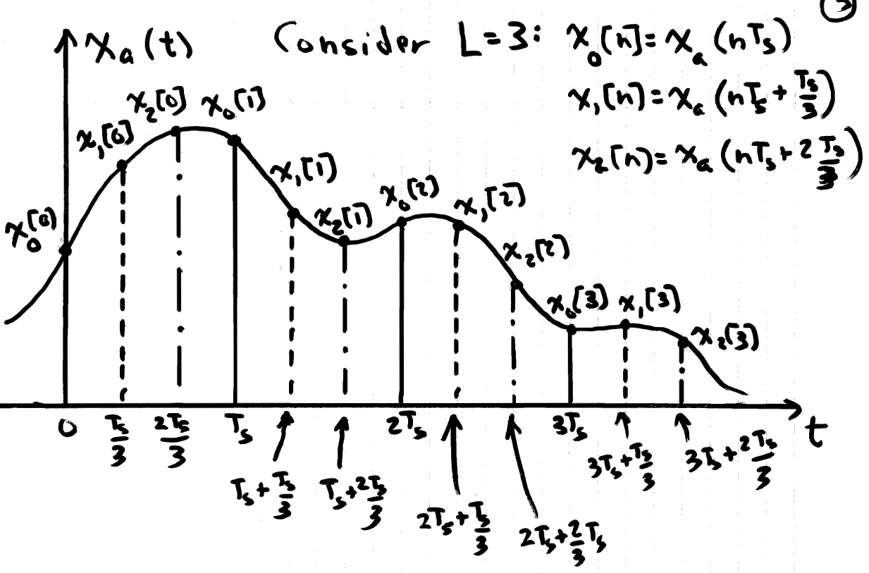
This can be further understood by referencing $x_a(t)$. $y_l[n]$ is given as

$$y_l[n]=x_a(\frac{nL+l}{L}T_s)=x_a(T_s(n+\frac{l}{L}))$$

The below figure visualizes the meaning of this relation. Each $y_l[n]$ is a sampling of $x_a(t)$ which starts at different multiples of $\frac{1}{L}$, in total constructing an upsampled version.

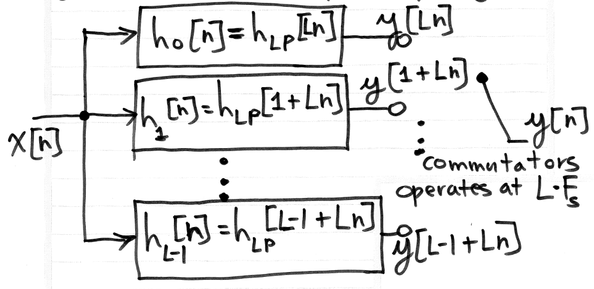
Each $y_l[n]$ is given by

$$y_l[n]=y[nL+l]=x[n]*h_{LP}[Ln+l]=x[n]*h_{l}[n]$$

This process is laid out schematically in the below figure:

2.2.1 “Polyphase Filters”

Fractional time shift filters are also called polyphase filters. This is because each $h_l[n]$ has linear phase, each with a different slope. To see this, assume an ideal LPF:

$$h_l[n]=\frac{sin(\pi(n+\frac{l}{L}))}{\pi(n+\frac{l}{L})}$$

Thus

$$H_l(\omega)=rect(\frac{\omega}{\pi})e^{j\frac{l}{L}\omega}$$

So each $h_l[n]$ has linear phase of $\frac{l}{L}\omega$.

3. Downsampling

The goal of digital downsampling is to acquire $x_a(DnT_s)$ from our samples of $x_a(nT_s)$ only. For now, let $L$ be an integer.

In short, we desire a digital system with relation

$$y[n] = x[Dn]$$

Although it won’t be proved here, the frequency domain relationship is

$$Y(\omega)=\frac{1}{D}\sum_{k=0}^{D-1}X(\frac{\omega - 2\pi k}{D})$$

The basic insight of this equation is that decimation expands the original signal’s bandwidth. The sum becomes important when aliasing occurs.