The purpose of this week is to understand digital subbanding and single-sideband modulation.

1. Digital SubBanding

The purpose of digital subbanding is to carry $L$ signals in one time-domain signal.

Since each signal can have bandwidth up to $\pi$, we must first compress the spectrums, modulate them to the appropriate bands, and then add the results.

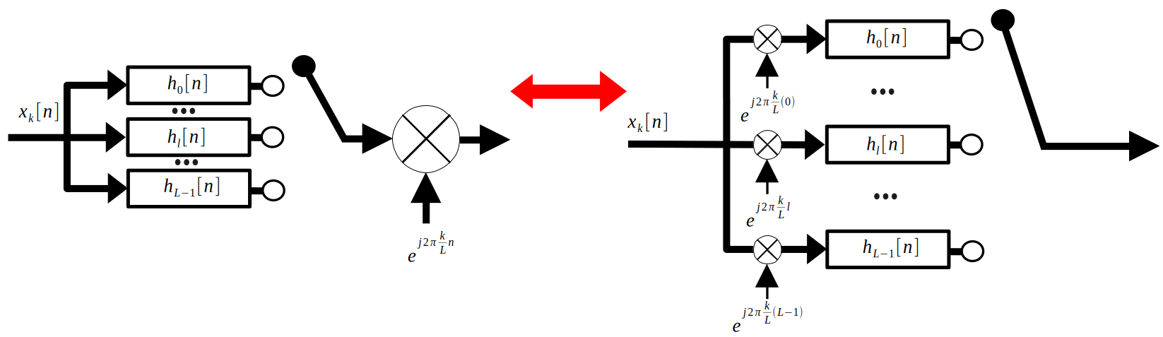
Using the naieve approach to upsampling, the below schematic representation of the process is created:

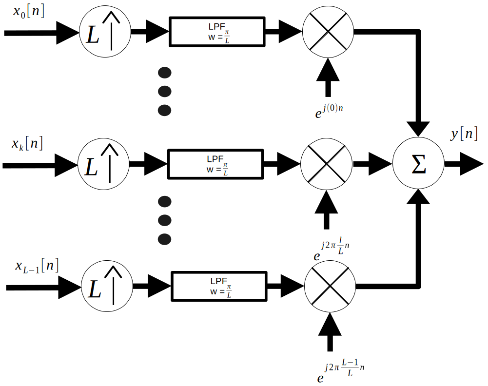
However, there is a much more efficient method. First, substitute the efficient method of upsampling into the diagram:

Since there is so much going on here, let’s focus on one input signal. Notice that by linearity, we can break the final modulating sine wave into each respective polyphase filter branch. Since the output of each filter branch only sees the cosine according to the frequency of the interleaver, we have to take into account the differences between each sine wave. The below figure shows the result.

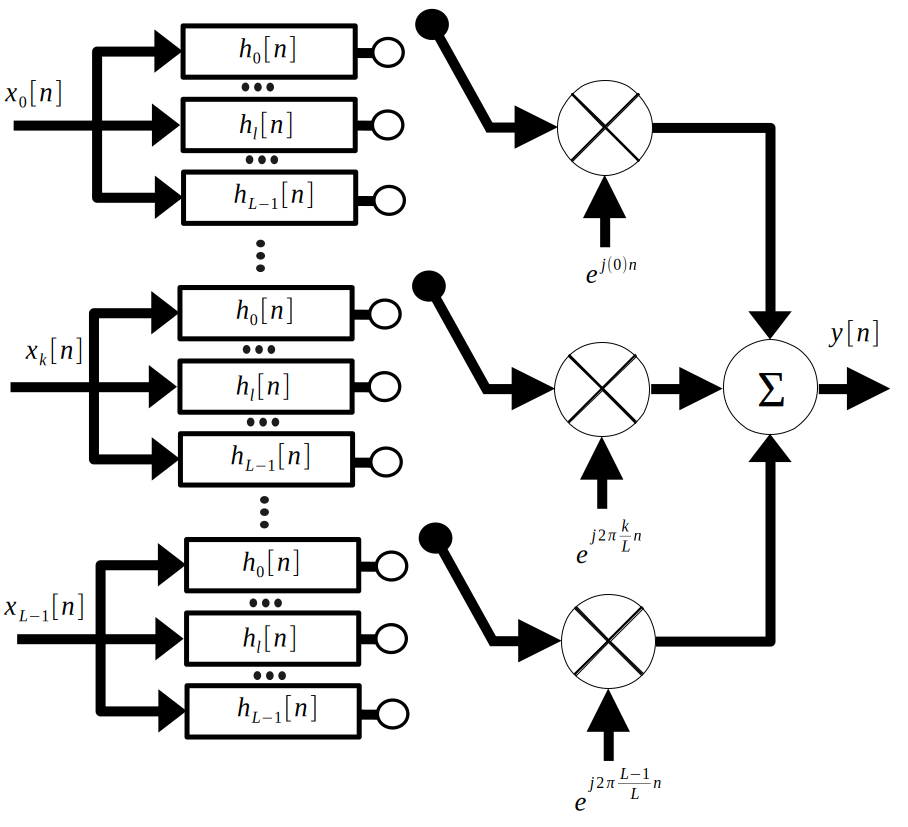
Finally, let’s look at the whole system, but only when the interleaver is connected to one polyphase filter branch. The lefthand side of the below figure shows this:

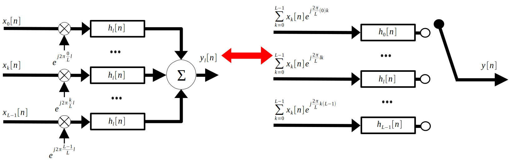
Reading the left hand side of the figure, we can see

$$y_l[n]=(\sum_{k=0}^{L-1}x_k[n]e^{j\frac{2\pi}{L}lk}*h_l[n])$$

With the distributive property, we see:

$$y_l[n]=h_l[n]*\sum_{k=0}^{L-1}x_k[n]e^{j\frac{2\pi}{L}lk}$$

Which is exactly what is shown for each polyphase branch in the right hand side of the above figure. To acquire $y[n]$ from $y_l[n]$, we interleave, as disucssed last week.

To succinctly summarize this system, we define:

$$ \mathbf{x}=\begin{bmatrix} x_0[n] \\ ... \\ x_k[n] \\ ... \\ x_{L-1}[n] \end{bmatrix} $$$$ \mathbf{a}=\begin{bmatrix} 1 & 1 & ... & 1\\ 1 & e^{j\frac{2\pi}{L}} & ... & e^{j\frac{2\pi}{L}(L-1)} \\ ... & ... & e^{j\frac{2\pi}{L}lk} & ... \\ 1 & ... & ... & e^{j\frac{2\pi}{L}(L-1)(L-1)} \\ \end{bmatrix} $$$$ \mathbf{h}=\begin{bmatrix} h_0[n] \\ ... \\ h_k[n] \\ ... \\ h_{L-1}[n] \end{bmatrix} $$$$ \mathbf{y}=\begin{bmatrix} y_0[n] \\ ... \\ y_k[n] \\ ... \\ y_{L-1}[n] \end{bmatrix} $$

These are related by

$$\mathbf{y}=(\mathbf{a}\mathbf{x}) .* \mathbf{h}$$

Where the $.*$ represents pointwise convolution.

2. SSB Modulation

In this context, the purpose of single side-band (SSB) modulation is to make a signal real-valued to improve the memory efficiency of modulated signals.

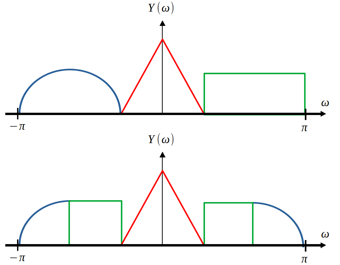
Recall that the fourier transform of a real valued signal obeys hemertian symmetry:

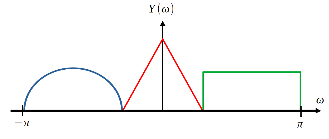
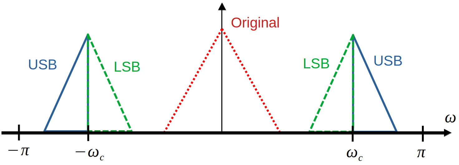
$$h(t) \in \mathbb{R} \Rightarrow H^*(\omega)=H(-\omega) \Rightarrow |H(\omega)|=|H(-\omega)|$$

So, upon observation of the below figure, it is clear that the top spectrum is a complex signal, which requires storing twice the amount of numbers as a real valued signal. Therefore, it is desirable to have the bottom spectrum, which is the purpose of SSB modulation.

First, some vocabulary: a DSB-SC modulated signal has two “bands,” the lower side band (LSB) and the upper side band (USB).

Let’s take the example of the USB for now. A feasible method of acquiring the USB is to pass it through a filter with a frequency response of the below rectangle:

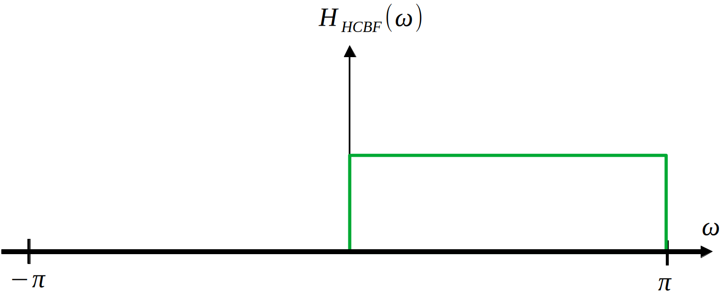
This filter can be expressed as

$$h_{HCBF}[n]=2\frac{sin(\frac{\pi}{2}n)}{\pi n}e^{j\frac{\pi}{2}}$$

Notice that this can be simplified into the following expression:

$$h_{HCBF}[n]=2\frac{sin(\frac{\pi}{2}n)}{\pi n}(cos(\frac{\pi}{2}n)+jsin(\frac{\pi}{2}n))=2\frac{sin(\frac{\pi}{2}n)}{\pi n}cos(\frac{\pi}{2}n)+j2\frac{sin(\frac{\pi}{2}n)}{\pi n}sin(\frac{\pi}{2}n)=\frac{sin(\pi n)}{\pi n}+j2\frac{sin^2(\frac{\pi}{2}n)}{\pi n}=\delta[n]+j2\frac{sin^2(\frac{\pi}{2}n)}{\pi n}$$

We shall examine the imaginary term of this expression. It is best to imagine this as a sinc pulse modulated by $sin(\frac{\pi}{2}n)$. Recall that this is $\frac{1}{2j}(\delta(\omega-\frac{\pi}{2})+\delta(\omega+\frac{\pi}{2}))$. Therefore, this term looks as follows:

We call this term the Hilbert transform. Thus, we have:

$$h_{HCBF}[n]=\delta[n]+jh_{HT}[n]$$

Now, let the output of this filter be:

$$\tilde{x}[n]=x[n]*h_{HCBF}[n]=x[n]+j\hat{x}[n]$$

With $\hat{x}[n]$ being the hilbert transform of $x[n]$

In order to make this signal real, it would be nice if we had a signal such as follows:

$$Z(\omega)=\frac{1}{2}[\tilde{X}(\omega)e^{j\omega_c n}+\tilde{X}^*(-\omega)e^{-j\omega_c n}]$$

Because this signal is exactly what we would like: a real-valued SSB signal.

Additionally, notice that:

$$Re\{x(t)\}=\frac{1}{2}[x(t)+x^*(t)]$$

$$\mathcal{F}\{x^*(t)\}=X^*(-\omega)$$

Thus, we desire

$$Re\{\tilde{x}[n]e^{j\omega_c n}\}=Re\{(x[n]+j\hat{x}[n])(cos(\omega_c n)+jsin(\omega_c n))\}=x[n]cos(\omega_c n) - \hat{x}[n]sin(\omega_c n)$$

Notice that this is an all-real term, and as such we have acquired what we wanted:

$$\boxed{z_{USB}[n]=[n]cos(\omega_c n) - \hat{x}[n]sin(\omega_c n)}$$

$$\boxed{z_{LSB}[n]=[n]cos(\omega_c n) + \hat{x}[n]sin(\omega_c n)}$$

The same procedure can be followed to obtain the LSB expression, where $h_{HCBF}[n]$ instead passes the negative frequencies, resulting in a sign change on the hilbert transform term.

3. Efficient SSB-Based Digital Subbanding

We now wish to construct a general method for subbanding $L$ signals with SSB modulation. In fact, we are one simple step yet from the proper implementation. Recall the efficient digital subbanding method described in section 1, summarized as

$$\mathbf{y}=(\mathbf{a}\mathbf{x}) .* \mathbf{h}$$

Section 2 has allowed us to make the $\mathbf{a}\mathbf{x}$ term into a real-valued signal.

In our notation, we want:

$$\mathbf{z}=Re\{\mathbf{a}\tilde{\mathbf{x}}\} .* \mathbf{h}$$

Writing this out in full:

$$ \begin{bmatrix} z_0[n] \\ ... \\ z_k[n] \\ ... \\ z_{L-1}[n] \end{bmatrix} = Re\{(\begin{bmatrix} 1 & 1 & ... & 1\\ 1 & cos(\frac{2\pi}{L}) & ... & cos(\frac{2\pi}{L}(L-1)) \\ ... & ... & cos(\frac{2\pi}{L}lk) & ... \\ 1 & ... & ... & cos(\frac{2\pi}{L}(L-1)(L-1)) \\ \end{bmatrix} +j\begin{bmatrix} 0 & 0 & ... & 0\\ 0 & sin(\frac{2\pi}{L}) & ... & sin(\frac{2\pi}{L}(L-1)) \\ ... & ... & sin(\frac{2\pi}{L}lk) & ... \\ 0 & ... & ... & sin(\frac{2\pi}{L}(L-1)(L-1)) \\ \end{bmatrix}) (\begin{bmatrix} x_0[n] \\ ... \\ x_k[n] \\ ... \\ x_{L-1}[n] \end{bmatrix} +j\begin{bmatrix} \hat{x}_0[n] \\ ... \\ \hat{x}_k[n] \\ ... \\ \hat{x}_{L-1}[n] \end{bmatrix})\} .* \begin{bmatrix} h_0[n] \\ ... \\ h_k[n] \\ ... \\ h_{L-1}[n] \end{bmatrix} $$

Let

$$ \mathbf{C}= \begin{bmatrix} 1 & 1 & ... & 1\\ 1 & cos(\frac{2\pi}{L}) & ... & cos(\frac{2\pi}{L}(L-1)) \\ ... & ... & cos(\frac{2\pi}{L}lk) & ... \\ 1 & ... & ... & cos(\frac{2\pi}{L}(L-1)(L-1)) \\ \end{bmatrix} $$

$$ \mathbf{S}=\begin{bmatrix} 0 & 0 & ... & 0\\ 0 & sin(\frac{2\pi}{L}) & ... & sin(\frac{2\pi}{L}(L-1)) \\ ... & ... & sin(\frac{2\pi}{L}lk) & ... \\ 0 & ... & ... & sin(\frac{2\pi}{L}(L-1)(L-1)) \\ \end{bmatrix} $$

$$ \hat{\mathbf{x}}=\begin{bmatrix} \hat{x}_0[n] \\ ... \\ \hat{x}_k[n] \\ ... \\ \hat{x}_{L-1}[n] \end{bmatrix} $$

Then we have

$$\boxed{\mathbf{z_{USB}}=(\mathbf{C}\mathbf{x}-\mathbf{S}\mathbf{\hat{x}}) .* \mathbf{h}}$$

$$\boxed{\mathbf{z_{LSB}}=(\mathbf{C}\mathbf{x}+\mathbf{S}\mathbf{\hat{x}}) .* \mathbf{h}}$$

4. Misc

There are actually many methods to generate SSB signals, especially for analog signals. The method covered here is called the “phase shift method,” since it makes use of using the hilbert transform to change the phase of an incoming signal. This method is shown schematically below. More of this is covered in ECE 440 notes.