ECE440 Week 2: DSB-SC Modulation
An introduction to Double SideBand - Suppressed Carrier (DSB-SC) modulation and various methods of generation.
1. Ideal DSB-SC
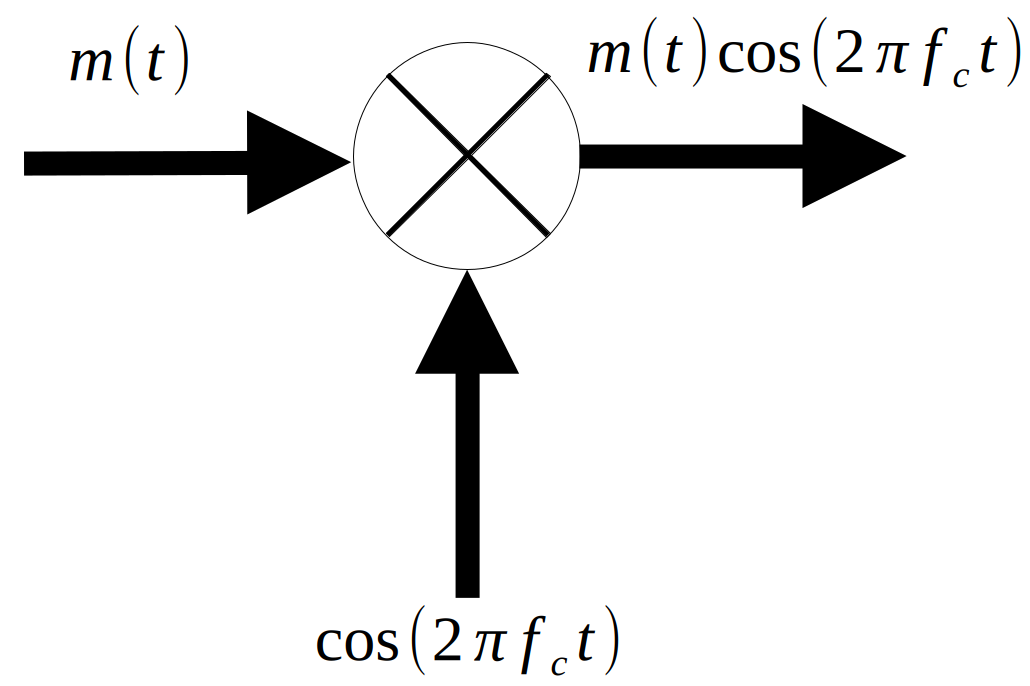
1.1 Ideal Modulation
The modulation of a DSB-SC signal is as simple as it gets - just multiply the message $m(t)$ by a sine wave, called the carrier. The frequency of the carrier is called, drumroll please, the carrier frequency $f_c$.
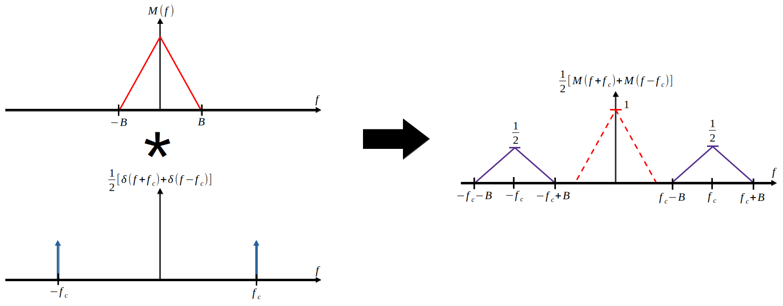
By the modulation property of the Fourier transform, it can be seen that the resulting waveform moves the message signal from the original baseband frequency range to a higher frequency range around the carrier frequency.
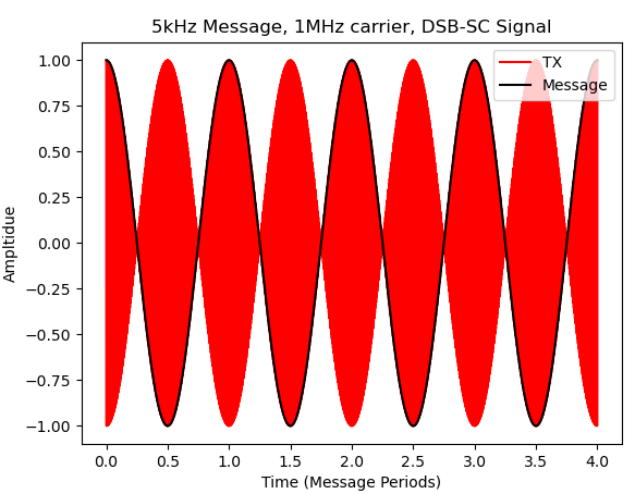
The below figures show what this modulation looks like in the time domain. The amplitude of the carrier can be seen varying as the message signal varies. This hints at a relationship with amplitude modulation (AM), and this relationship is in fact why we are bothering to study DSB-SC at all.
The first figure shows a DSB-SC signal with a carrier frequency of only 10x that of the message signal. As such, it is relatively easy to make out the carrier and message, but the carrier frequency of 50kHz still requires an antenna that is at least 1.5km long.

The second figure shows a much more realistic DSB-SC signal with a carrier at a frequency of 1MHz, which is right in the middle of the AM band in the USA. This brings our required antenna size down to 75m.
(Higher-power transmit antennae will be in the ballpark of 30m to 140m, but receive antennae don’t need to be so large. In fact, the FCC limits most AM antennae to being at most 3m long. For more discussion on this topic)
The third figure zooms in on one half period of the second to show that you can still make out the carrier.

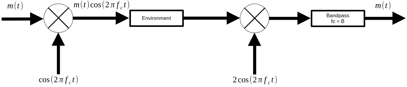
1.2 Ideal Demodulation
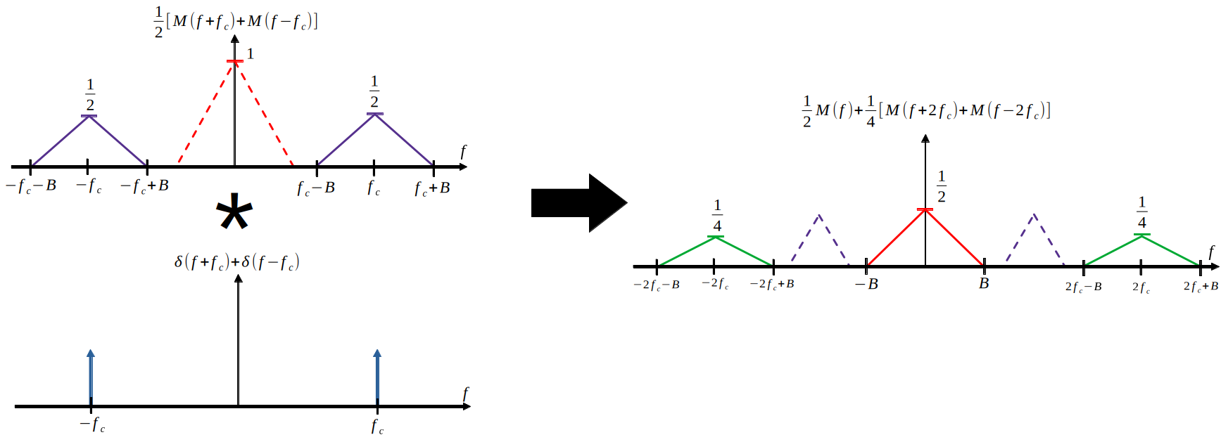
The demodulation of a DSB-SC signal is quite simple as well - multiply again by a sine wave of the carrier frequency, and pass the result through a band pass filter.

By applying the modulation property again, it can be seen that half of the original signal power is recovered in the baseband after multiplication by the carrier.
1.3 Circuit Implementation
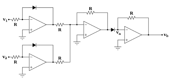
This circuit has transfer function:
$$v_b=v_1\cdot v_2$$And as such can be easily used to implement multiplication by the carrier.
2. Nonlinear DSB-SC Modulation
This method of modulation makes use of nonlinear circuit elements, such as a diode or transistor.
The transfer function of the nonlinear elements is approximated with a power series:
$$y_i(t)=ax_i(t)+bx_i(t)^2$$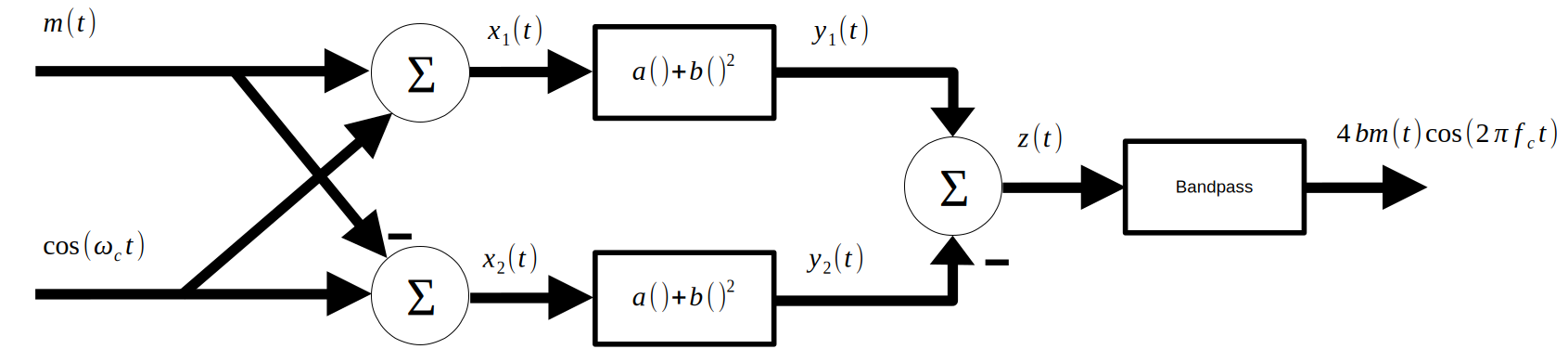
To analyze this system, work block-by-block:
$$x_1(t)=m(t)+cos(2\pi f_c t)$$$$x_2(t)=cos(2\pi f_c t)-m(t)$$
$$y_1(t)=a(m(t)+cos(2\pi f_c t))+b(m^2(t)+2m(t)cos(2\pi f_c t)+cos^2(2\pi f_c t))$$
$$y_2(t)=a(cos(2\pi f_c t)-m(t))+b(m^2(t)-2m(t)cos(2\pi f_c t)+cos^2(2\pi f_c t))$$
$$z(t)=2am(t)+4bm(t)cos(2\pi f_c t)$$
The BPF filters the $2am(t)$ term, leaving us with
$$4bm(t)cos(2\pi f_ct)$$3. Rectangular Carrier
The rectangular time-domain waveform with duty cycle $D$ and period $T_c$ can be expressed as
$$w(t) = \sum_{k=-\infty}^{\infty}rect(\frac{t-kT_c}{DT_c})$$Since $w(t)$ is a periodic and even function, we can write this waveform with a cosine fourier series:
$$w(t)=\sum_{k=0}^{\infty}w_kcos(2\pi kf_ct)$$When we use $w(t)$ as the carrier, we get
$$w(t)m(t)=\sum_{k=0}^{\infty}w_km(t)cos(2\pi kf_ct)$$Passing this through a bandpass filter, we obtain
$$w_1m(t)cos(2\pi kf_ct)$$Which we can then transmit.
3.1 Frequency Domain Analysis
By the modulation property:
$$\mathcal{F}\{w(t)m(t)\}=\sum_{k=0}^{\infty}\frac{w_k}{2}[M(f-kf_c)+M(f+kf_c)]$$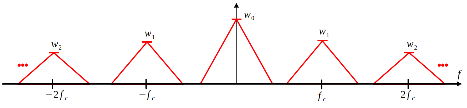
3.2 Time Domain Analysis
The below figures show what the time domain signals look like in this process:
The first figure shows the $w(t)m(t)$ signal and the original $m(t)$ signal.
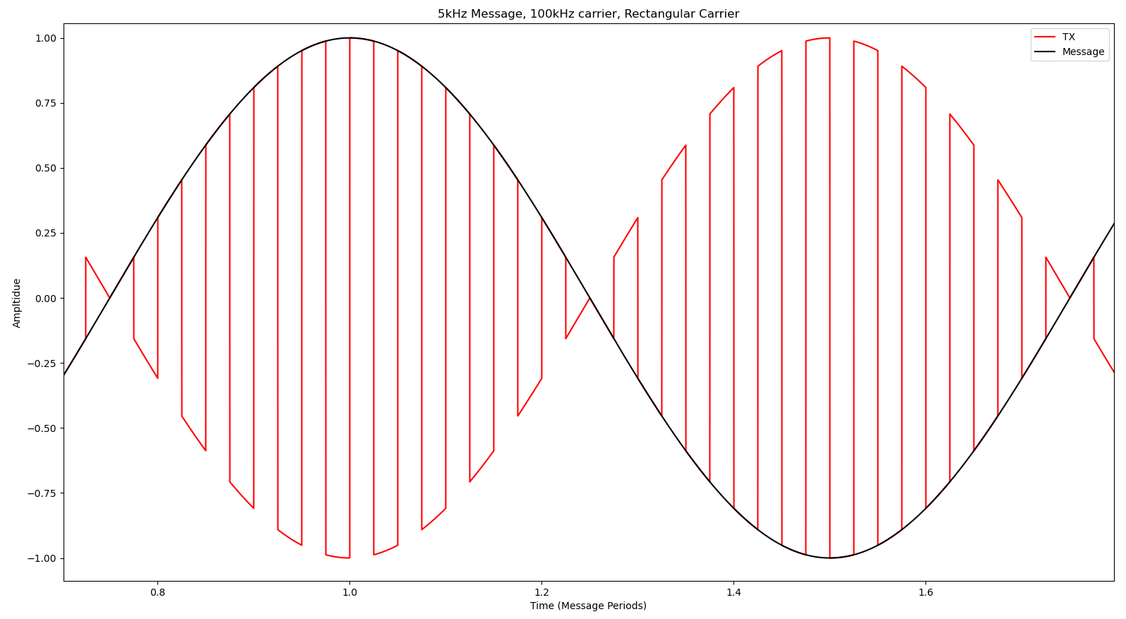
The second figure includes the carrier and scales the other two traces to make everything more visible.

The third figure shows the result of passing $w(t)m(t)$ through a bandpass filter. You can observe some delay due to the filter, and some distortion due to the inability to use a perfect filter.

4. Code
Below is the code used to generate the above plots.
    import matplotlib.pyplot as plt
    import numpy as np
    from scipy import signal
    from multipledispatch import dispatch

    @dispatch(np.ndarray,np.ndarray, np.ndarray, np.ndarray, str)
    def plotFunction(t,y1, y2, y3, title):
        plt.figure()
        plt.plot(t,y1, "r", label = "TX")
        plt.plot(t,y2, "k", label = "Message")
        plt.plot(t,y3, "b", label = "Carrier")
        plt.title(title)
        plt.legend(loc = "upper right")
        plt.xlabel("Time (Message Periods)")
        plt.ylabel("Ampltidue")
        plt.show()

    @dispatch(np.ndarray,np.ndarray, np.ndarray, str)
    def plotFunction(t,y1, y2, title):
        plt.figure()
        plt.plot(t,y1, "r", label = "TX")
        plt.plot(t,y2, "k", label = "Message")
        plt.title(title)
        plt.legend(loc = "upper right")
        plt.xlabel("Time (Message Periods)")
        plt.ylabel("Ampltidue")
        plt.show()

    @dispatch(np.ndarray,np.ndarray, str)
    def plotFunction(t,y, title):
        plt.figure()
        plt.plot(t,y, "r", label = "TX")
        plt.title(title)
        plt.xlabel("Time (Message Periods)")
        plt.ylabel("Ampltidue")
        plt.show()

    def ideal():
        fm = 5 * 10**3 # 5kHz
        fc = 1 * 10**6 # 1MHz
        t = np.linspace(0,4/fm,2*fc)
        T = np.linspace(0,4,2*fc)

        m = np.cos(2*np.pi*fm*t)
        c1 = np.cos(2*np.pi*fc*t)
        r1= m*c1

        plotFunction(T, r1, m, "5kHz Message, 1MHz carrier, DSB-SC Signal")

        fc = 50 * 10**3 # 50kHz
        c2 = np.cos(2*np.pi*fc*t)
        r2 = m*c2

        plotFunction(T, r2, m, "5kHz Message, 50kHz carrier, DSB-SC Signal")

    def rectangle():
        # need to change frequencies to lower bound so nyquist rate is lower and therefore convolution doesn't take so long
        fm = 5 # 5Hz
        fc = 100 # 100Hz
        Fs = 10*fc
        T = np.linspace(0,4,Fs)
        t = np.linspace(-400,400,Fs)

        m = np.cos(2*np.pi*fm*t)
        c = signal.square(2*np.pi*fc*t)
        r= m*c

        plotFunction(T, r, m, "5kHz Message, 100kHz carrier, Rectangular Carrier")
        plotFunction(T, r, m, 0.5*c, "5kHz Message, 100kHz carrier, Rectangular Carrier")

        h = np.sin(2*np.pi*(fm/Fs)*t)/(np.pi*t)*np.sin(2*np.pi*(fc/Fs)*t) # bandpass by sinc and modulation property

        plotFunction(t,h,"Filter impulse response")

        y = np.convolve(r,h) # put through filter

        margin = len(y)-len(t)
        y1 = y[margin//2:len(y)-margin//2 - 1]

        plotFunction(T,y1,m,"filter output")

    ideal()
    rectangle()

    print("done")