Topics and concepts covered in weeks 6-9 of ECE538 at Purdue University.

CTFT

Definition

The CTFT of a signal $x(t)$ is defined as follows:

$$X(f) = \int_{t=-\infty}^{\infty}x(t)e^{-j2\pi ft}dt$$

The inverse CTFT is given as:

$$x(t)=\int_{f=-\infty}^{\infty}X(f)e^{j2\pi ft}df$$

Some quick notes:

• Notice that we are not using the $X(jw)$ notation
• Notice that we are in Hz, not rad/s. Things are much prettier this way :)

Side note:

This can be viewed as a projection of $x(t)$ onto $e^{j2\pi ft}$ in a Hilbert space with inner product $\langle x,y \rangle$ given as:

$$\langle x(t),y(t) \rangle=\int_{t=-\infty}^{\infty}x(t)y^*(t)dt$$

Properties

Duality

From the definition of the CTFT, we can immediately obtain the following relation:

$$x(t) \overset{\mathcal{F}}{\leftrightarrow} X(f) \iff X(t) \overset{\mathcal{F}}{\leftrightarrow} x(-f)$$

This is a useful property for obtaining many other properties.

Proof

Start with

$$X(f) = \int_{t=-\infty}^{\infty}x(t)e^{-j2\pi ft}dt \equiv x(t) \overset{\mathcal{F}}{\leftrightarrow} X(f)$$

Rewrite the fourier transform with $f=z$, $t=y$

$$X(z) = \int_{y=-\infty}^{\infty}x(y)e^{-j2\pi yz}dy$$

Now rewrite with $y = -f$ and $z = t$

$$X(t)=\int_{f=-\infty}^{\infty}x(-f)e^{j2\pi ft}df \equiv X(t) \overset{\mathcal{F}}{\leftrightarrow} x(-f)$$

This means that

$$x(t) \overset{\mathcal{F}}{\leftrightarrow} X(f) \iff X(t) \overset{\mathcal{F}}{\leftrightarrow} x(-f)$$$$\fbox{QED}$$

Linearity

It’s worth stating explicitly, but… duh…

$$a_1x_1(t)+a_2x_2(t) \overset{\mathcal{F}}{\leftrightarrow} a_1X_1(f)+a_2X_2(f)$$

Time Scaling

This is a very useful property for conceptual understanding.

$$x(at) \overset{\mathcal{F}}{\leftrightarrow} \frac{1}{|a|}X(\frac{f}{a})$$

As you can see, if you scale a signal horizontally in the time domain, the opposite occurs in the frequency domain.

This leads to a nice conceptual principle: $\fbox{The shorter the signal in time, the wider the signal in frequency.}$

And by duality, vice a versa.

Conjugation

$$x^*(t) \overset{\mathcal{F}}{\leftrightarrow} X^*(-f)$$

Convolution/Multiplication

This is our first dual pair of properties. This means that once one result is achieved, the other can easily be through duality.

$$x_1(t)*x_2(t) \overset{\mathcal{F}}{\leftrightarrow} X_1(f)X_2(f)$$

$$x_1(t)\cdot x_2(t) \overset{\mathcal{F}}{\leftrightarrow} X_1(f)*X_2(f)$$

Proof

$$\mathcal{F}\{x_1(t)*x_2(t)\}=\mathcal{F}\{\int_{\lambda=-\infty}^{\infty}x_1(\lambda)x_2(t-\lambda)d\lambda\}=\int_{\lambda=-\infty}^{\infty}x_1(\lambda)\mathcal{F}\{x_2(t-\lambda)\}d\lambda$$$$\mathcal{F}\{x_2(t-\lambda)\}=\int_{t=-\infty}^{\infty}x_2(t-\lambda)e^{-j2\pi ft}dt$$

Let $u = t-\lambda$

$$\int_{t=-\infty}^{\infty}x_2(t-\lambda)e^{-j2\pi ft}dt = e^{-j2\pi f\lambda}\int_{u=-\infty}^{\infty}x_2(u)e^{-j2\pi fu}du = e^{-j2\pi f\lambda}X_2(f)$$

Thus

$$\int_{\lambda=-\infty}^{\infty}x_1(\lambda)\mathcal{F}\{x_2(t-\lambda)\}d\lambda=X_2(f)\int_{\lambda=-\infty}^{\infty}x_1(\lambda)e^{-j2\pi f\lambda}d\lambda = X_1(f)X_2(f)$$

Therefore

$$\mathcal{F}\{x_1(t)*x_2(t)\} = X_1(f)X_2(f)$$$$\fbox{QED pt 1}$$

By duality:

$$X_1(t)\cdot X_2(t) \overset{\mathcal{F}}{\leftrightarrow} \int_{\lambda=-\infty}^{\infty} x_1(\lambda)x_2(-f-\lambda)d\lambda$$

Let $\lambda = f - u$

$$\int_{\lambda=-\infty}^{\infty} x_1(\lambda)x_2(-f-\lambda)d\lambda = -\int_{u=\infty}^{-\infty} x_1(f - u)x_2(u)du$$

(at this point, we could invoke commutativity of convolution and be done with it. However, we can push to the end)

Now let $u = f - v$

$$-\int_{u=\infty}^{-\infty} x_1(f - u)x_2(u)du = \int_{v=-\infty}^{\infty} x_1(v)x_2(f-v)dv = x_1(f)*x_2(f)$$

Therefore

$$\mathcal{F}\{x_1(t)x_2(t)\} = X_1(f)*X_2(f)$$$$\fbox{QED pt 2}$$

Complex Sinusoid / Delta

A fundamental pair:

$$\delta(t-t_0) \overset{\mathcal{F}}{\leftrightarrow} e^{-j2\pi ft_0}$$

$$e^{j2\pi f_ct} \overset{\mathcal{F}}{\leftrightarrow} \delta(f-f_c)$$

Proof

Notice that we cannot attempt $\mathcal{F}\{e^{j2\pi f_ct}\}$ directly, as $e^{j2\pi f_ct}$ has infinite energy. However, we can take the other route and use duality to obtain the other.

$$\mathcal{F}\{\delta(t-t_0)\}=\int_{t=-\infty}^{\infty}\delta(t-t_0)e^{-j2\pi ft}dt=\int_{t=-\infty}^{\infty}\delta(t-t_0)e^{-j2\pi ft_0}dt=e^{-j2\pi ft_0}\int_{t=-\infty}^{\infty}\delta(t-t_0)dt=e^{-j2\pi ft_0}$$

Therefore,

$$\mathcal{F}\{\delta(t-t_0)\}=e^{-j2\pi ft_0}$$$$\fbox{QED pt 1}$$

Also notice

$$\mathcal{F}\{\delta(t+t_0)\}=e^{j2\pi ft_0}$$

By duality, ($f_c = t_0$)

$$\mathcal{F}\{e^{j2\pi f_ct}\}=\delta(-f+f_c)=\delta(f-f_c)$$$$\fbox{QED pt 2}$$

Time/Frequency Shifting

The below properties can be derived with a combination of the convolution property and duality.

$$x(t)e^{j2\pi f_ct} \overset{\mathcal{F}}{\leftrightarrow} X(f-f_c)$$

$$x(t-t_0) \overset{\mathcal{F}}{\leftrightarrow} X(f)e^{-j2\pi ft_0}$$

1. CTFT, DTFT Relationship

1.1 Prerequisites

First, we shall establish some variables and concepts.

Let $x_a(t)$ be the analog signal to be sampled into $x[n]$ by $x_s(t)$ with a sampling frequency $F_s=\frac{1}{T_s}$. The relationships between these variables are:

$$x[n]=x_a(nT_s)$$

$$x_s(t)=x_a(t)\sum_{n=-\infty}^{\infty}\delta(t-nT_s)$$

DTFT:

$$X(\omega)=\sum_{n=-\infty}^{\infty}x[n]e^{-j\omega n}$$

CTFT:

$$X_a(\omega)=\int_{t=-\infty}^{\infty}x_a(t)e^{-j\omega t}dt$$

The relationship between $x_s(t)$ and $x[n]$ is the central topic we’d like to discuss.

1.2 Derivation

First, notice the following:

$$x_s(t)=x_a(t)\sum_{n=-\infty}^{\infty}\delta(t-nT_s) \Rightarrow X_s(\omega) = X_a(\omega)*F_s\sum_{n=-\infty}^{\infty}\delta(\omega-2\pi nF_s)$$

$$X_s(\omega) = F_s\sum_{n=-\infty}^{\infty}X_a(\omega-2\pi nF_s)$$

Hold this in your pocket, we now move on. From the following:

$$x_s(t)=x_a(t)\sum_{n=-\infty}^{\infty}\delta(t-nT_s)=\sum_{n=-\infty}^{\infty}x_a(nT_s)\delta(t-nT_s)$$

$$X_s(\omega) = \sum_{n=-\infty}^{\infty}x_a(nT_s)e^{-j\omega nT_s}=\sum_{n=-\infty}^{\infty}x[n]e^{-j\omega nT_s}$$

Now perform the following substitution:

$$\boxed{X_s(\omega F_s) = \sum_{n=-\infty}^{\infty}x[n]e^{-j\omega n F_sT_s}=\sum_{n=-\infty}^{\infty}x[n]e^{-j\omega n}=X(\omega)}$$

1.3 Interpretation

To interpret this result, notice that the input to $X_s(\omega)$ can be called the analog frequency, $\omega_a$ and the input to $X(\omega)$ can be called the digital frequency, $\omega_d$. Therefore, we have

$$\omega_a=\omega_d F_s$$

Another note of importance is that $X_s(\omega F_s) = X(\omega)$, combined with the fact that

$$X_s(\omega) = F_s\sum_{n=-\infty}^{\infty}X_a(\omega-2\pi nF_s)$$

Means

$$X(\omega) = F_s\sum_{n=-\infty}^{\infty}X_a(\omega F_s-2\pi nF_s)=F_s\sum_{n=-\infty}^{\infty}X_a(F_s(\omega -2\pi n))$$

Which means that the DTFT takes the analog spectrum and compressed it by $F_s$, then repeats it at every mutliple of $2\pi$ and adds the result. Notice that this explains aliasing - if $F_s$ is too small, the compression does not prevent overlapping of neighboring spectra.

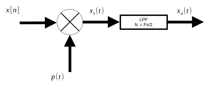
2. Ideal Reconstruction, or D2A Conversion

In order to reconstruct $x_a(t)$ from $x[n]$, we use $x_s(t)$:

$$x_s(t) = \sum_{n=-\infty}^{\infty}x[n]\delta(t-nT_s)$$$$X_s(f) = F_s\sum_{n=-\infty}^{\infty}X_a(f- nF_s)$$

As can be seen, if you pass $x_s(t)$ into a low pass filter, then you can retrieve $x_a(t)$.

1. Reconstruction (D2A Conversion)

The below figure represents the D2A conversion process in blocks. We first focus on the LPF, then the upsampler.

1.1 Ideal Reconstruction Filters

Recall that we have

$$X_s(f) = F_s\sum_{n=-\infty}^{\infty}X_a(f- nF_s)$$

And thus a LPF centered around the first copy of $X_a(f)$ is used to recover $x_a(t)$.

The first LPF to consider is a simple rectangle. However, notice that the time domain signal required for this rectangle is an infinite-length sinc wave. Major distortion in the form of Gibb’s phenomenon is present when truncating the signal for practical applications, thus we search for better alternatives.

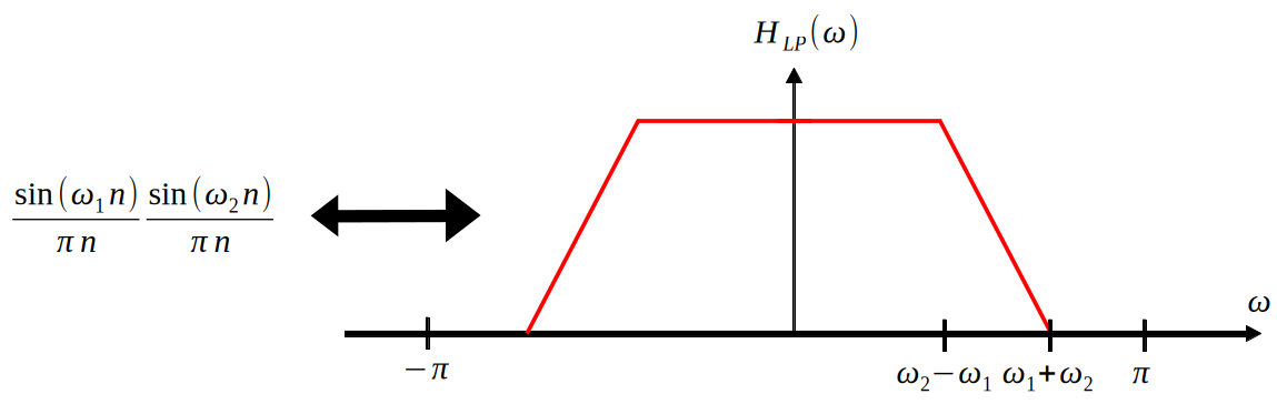
The next LPF to consider is inspired by the first - by moving from $sinc(t)$ to $sinc^2(t)$. Consider that $sinc^2(t)$ has a more signal power concentrated near the center of the wave than simple $sinc(t)$ does, therefore this seems promising. However, remember that $sinc^2(t)$ gives a triangle in the frequency domain, which does not preserve the property that the baseband $X_a(f)$ is preserved after the filter. Therefore, the below solution is chosen - by convolving two rectangles of different widths, we achieve the desired result.

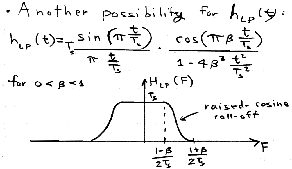
The final LPF to consider is the raised cosine filter. This also has the desired properties for reconstruction.

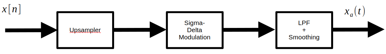
1.2 Use of Upsampling in Reconstruction

In order to understand why upsampling is used in the reconstruction process, we must first understand the sigma-delta modulator. In short, sigma-delta modulation is an efficienct scheme for A2D and D2A conversion that changes its output level only one quantization level at a time by comparing the current value to the desired value and updating accordingly. The below figure illustrates this behavior - initially, the SDM output is 0, but it climbs at each step until it reaches the steady state of the analog signal.

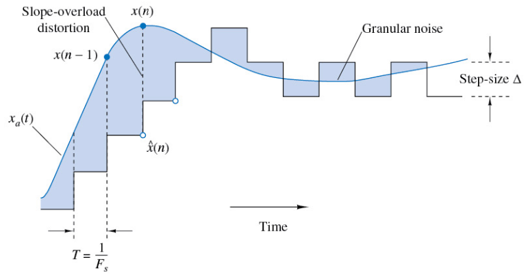
Upsampling is used before this process because SDM is a much more accurate process the quicker you sample. So, if we can somehow digitally change the sampling frequency, we can make D2A a much more accurate process.

2. Upsampling

The goal of digital upsampling is to acquire $x_a(\frac{nT_s}{L})$ from our samples of $x_a(nT_s)$ only. For now, let $L$ be an integer.

In short, we desire a digital system with relation

$$y[n] = x[\frac{n}{L}] = \sum_{k=-\infty}^{\infty}x[k]\delta[n-kL]$$

Notice that in the frequency domain, the relation is

$$Y(\omega)=X(L\omega)$$

This is useful in digital subbanding

2.1 Inefficient Method - Zero Inserts

Recall that through the process of reconstruction, we obtain:

$$x_a(t)=[\sum_{k=-\infty}^{\infty}x[k]\delta(t-kT_s)]*h_{LP}(t)$$

We wish to obtain

$$y[n]=x_a(\frac{nTs}{L})=[\sum_{k=-\infty}^{\infty}x[k]\delta[\frac{n}{L}-k]]*h_{LP}[\frac{n}{L}]$$

Which amounts to

$$y[n]=x_a(\frac{nTs}{L})=x[\frac{n}{L}]*h_{LP}[\frac{n}{L}]$$

This is schematically represented in the below figure.

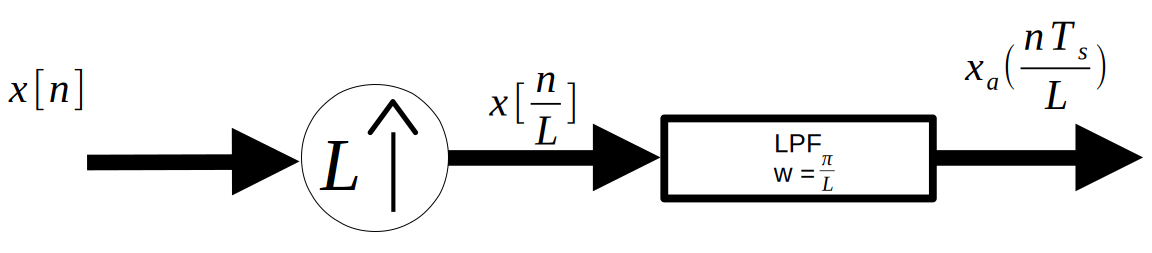
The $x[\frac{n}{L}]$ term is represented by the circle with an L inside of it. This element inserts $L-1$ zeros in between each sample of $x[n]$. Thus, the function of the LPF can be seen as “filling in” those zeros through convolution.

However, this means that this process is incredibly inefficienct, as most of the convolution performed when passing the zero-insert output into the LPF is just multiplication by 0. We hunt for a more efficient version in the rest of this chapter.

2.2 Efficient Method - Fractional Time Shift Filters

First, notice that $y[n]$ can be written as below:

$$y[n]=\sum_{k=-\infty}^{\infty}x[k]h_{LP}[n-Lk]$$

This is very close to convolution. How could we make this convolution?

$$y[Ln] = \sum_{k=-\infty}^{\infty}x[k]h_{LP}[L(n-k)]=x[n]*h_{LP}[Ln]$$

Now notice that $y[Ln]$ gives every $L-1$ element of y[n] starting at $n=0$. If we shift this by 1, we should get every $L-1$ element starting at $n=1$, and we can repeat this process up to the $L-1$ element.

Let

$$y_l[n]=y[nL+l]$$

Then we can reconstruct $y[n]$ by interleaving each $y_l[n]$ one after the other into $y[n]$, starting at $l=0$ and moving up to $l=L-1$.

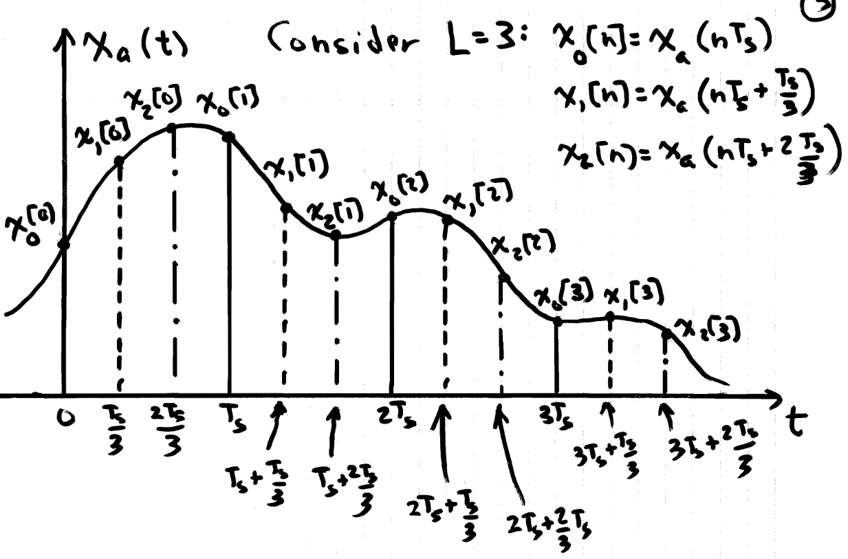
This can be further understood by referencing $x_a(t)$. $y_l[n]$ is given as

$$y_l[n]=x_a(\frac{nL+l}{L}T_s)=x_a(T_s(n+\frac{l}{L}))$$

The below figure visualizes the meaning of this relation. Each $y_l[n]$ is a sampling of $x_a(t)$ which starts at different multiples of $\frac{1}{L}$, in total constructing an upsampled version.

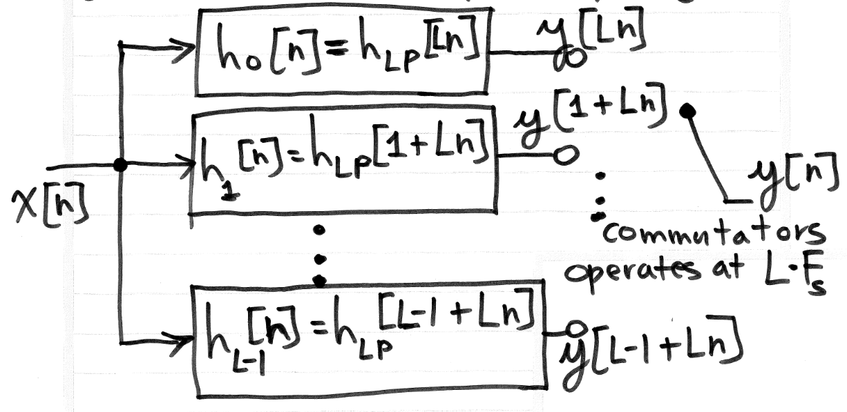
Each $y_l[n]$ is given by

$$y_l[n]=y[nL+l]=x[n]*h_{LP}[Ln+l]=x[n]*h_{l}[n]$$

This process is laid out schematically in the below figure:

2.2.1 “Polyphase Filters”

Fractional time shift filters are also called polyphase filters. This is because each $h_l[n]$ has linear phase, each with a different slope. To see this, assume an ideal LPF:

$$h_l[n]=\frac{sin(\pi(n+\frac{l}{L}))}{\pi(n+\frac{l}{L})}$$

Thus

$$H_l(\omega)=rect(\frac{\omega}{\pi})e^{j\frac{l}{L}\omega}$$

So each $h_l[n]$ has linear phase of $\frac{l}{L}\omega$.

3. Downsampling

The goal of digital downsampling is to acquire $x_a(DnT_s)$ from our samples of $x_a(nT_s)$ only. For now, let $L$ be an integer.

In short, we desire a digital system with relation

$$y[n] = x[Dn]$$

Although it won’t be proved here, the frequency domain relationship is

$$Y(\omega)=\frac{1}{D}\sum_{k=0}^{D-1}X(\frac{\omega - 2\pi k}{D})$$

The basic insight of this equation is that decimation expands the original signal’s bandwidth. The sum becomes important when aliasing occurs.

1. Digital SubBanding

The purpose of digital subbanding is to carry $L$ signals in one time-domain signal.

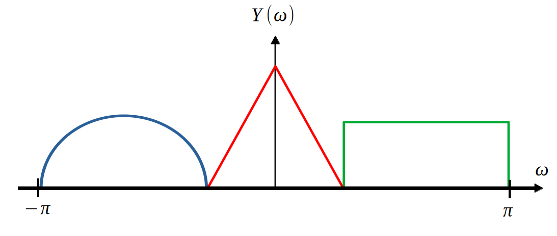
Since each signal can have bandwidth up to $\pi$, we must first compress the spectrums, modulate them to the appropriate bands, and then add the results.

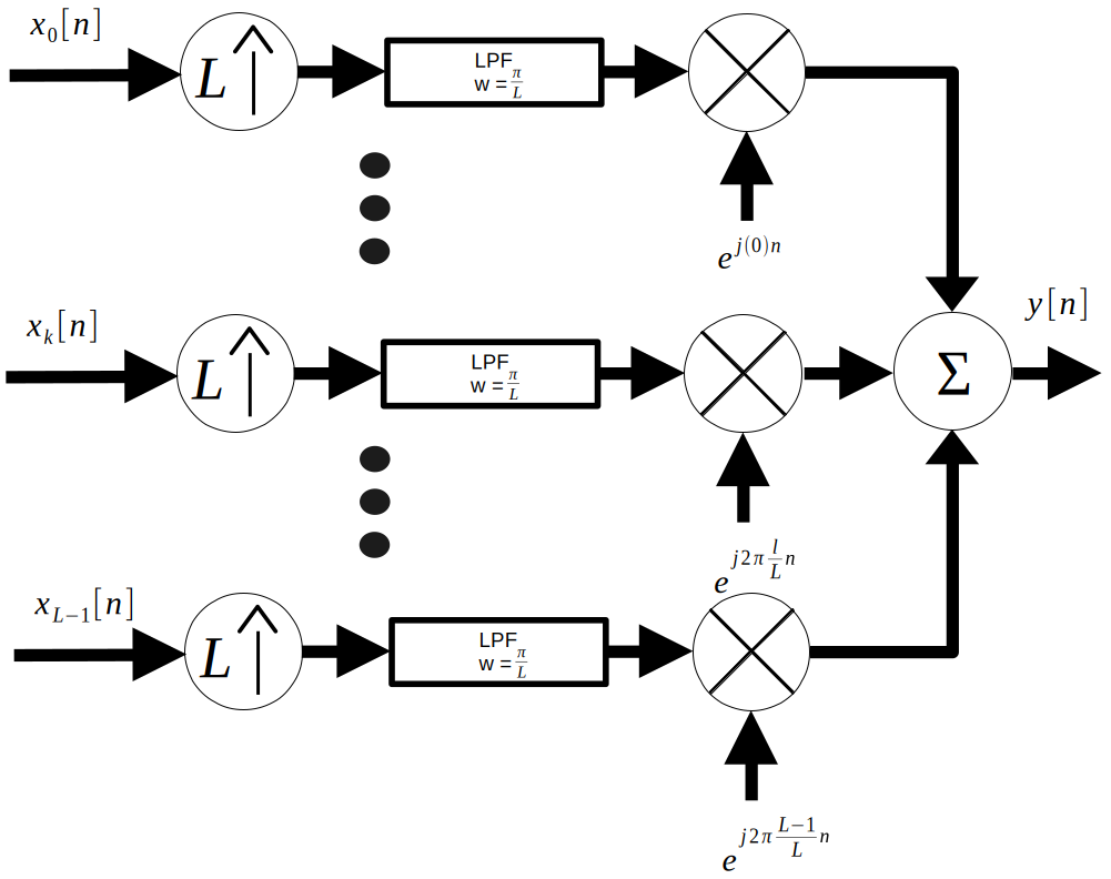
Using the naieve approach to upsampling, the below schematic representation of the process is created:

However, there is a much more efficient method. First, substitute the efficient method of upsampling into the diagram:

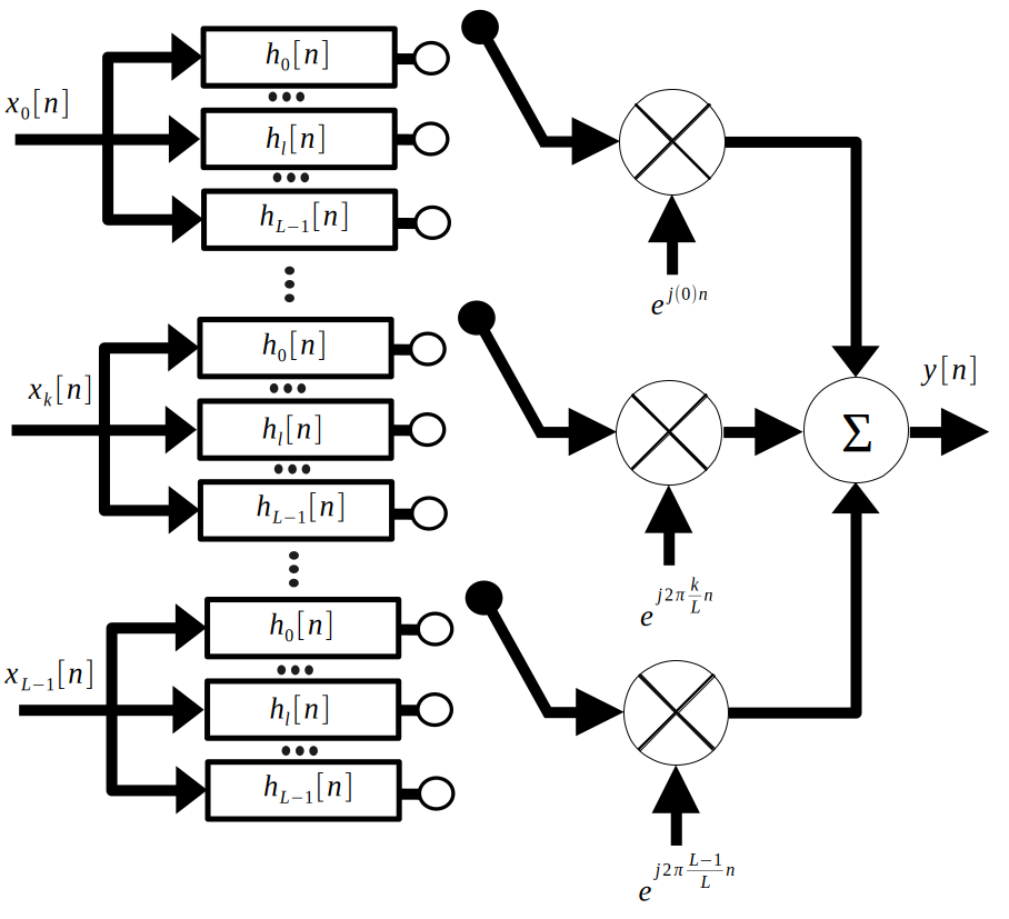
Since there is so much going on here, let’s focus on one input signal. Notice that by linearity, we can break the final modulating sine wave into each respective polyphase filter branch. Since the output of each filter branch only sees the cosine according to the frequency of the interleaver, we have to take into account the differences between each sine wave. The below figure shows the result.

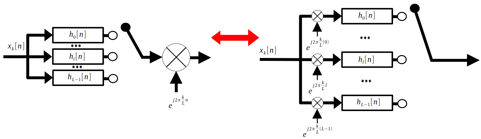
Finally, let’s look at the whole system, but only when the interleaver is connected to one polyphase filter branch. The lefthand side of the below figure shows this:

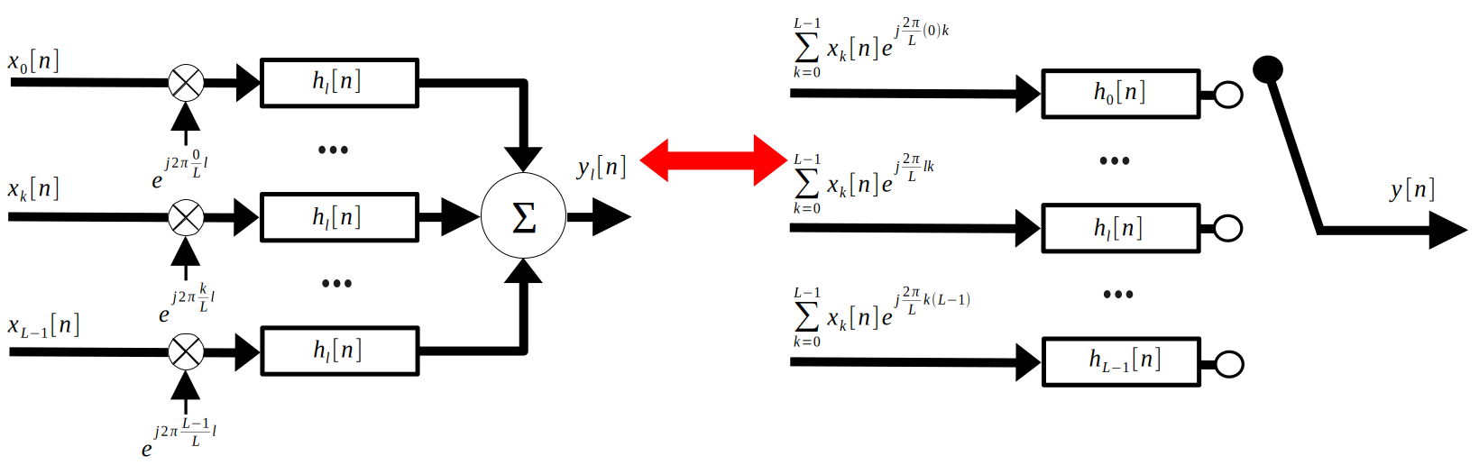
Reading the left hand side of the figure, we can see

$$y_l[n]=(\sum_{k=0}^{L-1}x_k[n]e^{j\frac{2\pi}{L}lk}*h_l[n])$$

With the distributive property, we see:

$$y_l[n]=h_l[n]*\sum_{k=0}^{L-1}x_k[n]e^{j\frac{2\pi}{L}lk}$$

Which is exactly what is shown for each polyphase branch in the right hand side of the above figure. To acquire $y[n]$ from $y_l[n]$, we interleave, as disucssed last week.

To succinctly summarize this system, we define:

$$ \mathbf{x}=\begin{bmatrix} x_0[n] \\ ... \\ x_k[n] \\ ... \\ x_{L-1}[n] \end{bmatrix} $$$$ \mathbf{a}=\begin{bmatrix} 1 & 1 & ... & 1\\ 1 & e^{j\frac{2\pi}{L}} & ... & e^{j\frac{2\pi}{L}(L-1)} \\ ... & ... & e^{j\frac{2\pi}{L}lk} & ... \\ 1 & ... & ... & e^{j\frac{2\pi}{L}(L-1)(L-1)} \\ \end{bmatrix} $$$$ \mathbf{h}=\begin{bmatrix} h_0[n] \\ ... \\ h_k[n] \\ ... \\ h_{L-1}[n] \end{bmatrix} $$$$ \mathbf{y}=\begin{bmatrix} y_0[n] \\ ... \\ y_k[n] \\ ... \\ y_{L-1}[n] \end{bmatrix} $$

These are related by

$$\mathbf{y}=(\mathbf{a}\mathbf{x}) .* \mathbf{h}$$

Where the $.*$ represents pointwise convolution.

2. SSB Modulation

In this context, the purpose of single side-band (SSB) modulation is to make a signal real-valued to improve the memory efficiency of modulated signals.

Recall that the fourier transform of a real valued signal obeys hemertian symmetry:

$$h(t) \in \mathbb{R} \Rightarrow H^*(\omega)=H(-\omega) \Rightarrow |H(\omega)|=|H(-\omega)|$$

So, upon observation of the below figure, it is clear that the top spectrum is a complex signal, which requires storing twice the amount of numbers as a real valued signal. Therefore, it is desirable to have the bottom spectrum, which is the purpose of SSB modulation.

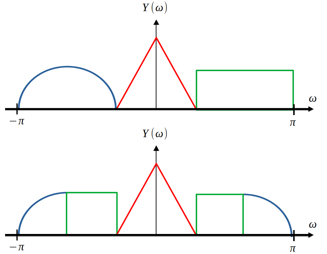
First, some vocabulary: a DSB-SC modulated signal has two “bands,” the lower side band (LSB) and the upper side band (USB).

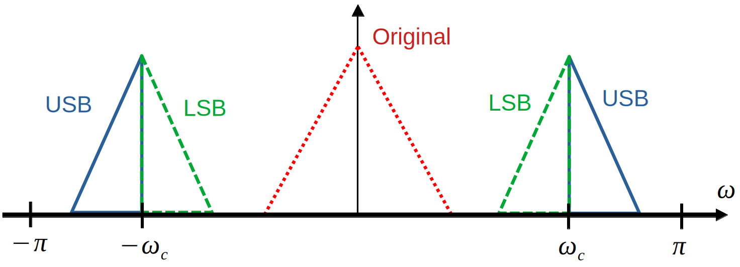
Let’s take the example of the USB for now. A feasible method of acquiring the USB is to pass it through a filter with a frequency response of the below rectangle:

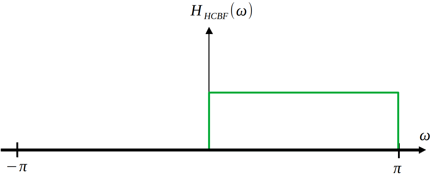
This filter can be expressed as

$$h_{HCBF}[n]=2\frac{sin(\frac{\pi}{2}n)}{\pi n}e^{j\frac{\pi}{2}}$$

Notice that this can be simplified into the following expression:

$$h_{HCBF}[n]=2\frac{sin(\frac{\pi}{2}n)}{\pi n}(cos(\frac{\pi}{2}n)+jsin(\frac{\pi}{2}n))=2\frac{sin(\frac{\pi}{2}n)}{\pi n}cos(\frac{\pi}{2}n)+j2\frac{sin(\frac{\pi}{2}n)}{\pi n}sin(\frac{\pi}{2}n)=\frac{sin(\pi n)}{\pi n}+j2\frac{sin^2(\frac{\pi}{2}n)}{\pi n}=\delta[n]+j2\frac{sin^2(\frac{\pi}{2}n)}{\pi n}$$

We shall examine the imaginary term of this expression. It is best to imagine this as a sinc pulse modulated by $sin(\frac{\pi}{2}n)$. Recall that this is $\frac{1}{2j}(\delta(\omega-\frac{\pi}{2})+\delta(\omega+\frac{\pi}{2}))$. Therefore, this term looks as follows:

We call this term the Hilbert transform. Thus, we have:

$$h_{HCBF}[n]=\delta[n]+jh_{HT}[n]$$

Now, let the output of this filter be:

$$\tilde{x}[n]=x[n]*h_{HCBF}[n]=x[n]+j\hat{x}[n]$$

With $\hat{x}[n]$ being the hilbert transform of $x[n]$

In order to make this signal real, it would be nice if we had a signal such as follows:

$$Z(\omega)=\frac{1}{2}[\tilde{X}(\omega)e^{j\omega_c n}+\tilde{X}^*(-\omega)e^{-j\omega_c n}]$$

Because this signal is exactly what we would like: a real-valued SSB signal.

Additionally, notice that:

$$Re\{x(t)\}=\frac{1}{2}[x(t)+x^*(t)]$$

$$\mathcal{F}\{x^*(t)\}=X^*(-\omega)$$

Thus, we desire

$$Re\{\tilde{x}[n]e^{j\omega_c n}\}=Re\{(x[n]+j\hat{x}[n])(cos(\omega_c n)+jsin(\omega_c n))\}=x[n]cos(\omega_c n) - \hat{x}[n]sin(\omega_c n)$$

Notice that this is an all-real term, and as such we have acquired what we wanted:

$$\boxed{z_{USB}[n]=[n]cos(\omega_c n) - \hat{x}[n]sin(\omega_c n)}$$

$$\boxed{z_{LSB}[n]=[n]cos(\omega_c n) + \hat{x}[n]sin(\omega_c n)}$$

The same procedure can be followed to obtain the LSB expression, where $h_{HCBF}[n]$ instead passes the negative frequencies, resulting in a sign change on the hilbert transform term.

3. Efficient SSB-Based Digital Subbanding

We now wish to construct a general method for subbanding $L$ signals with SSB modulation. In fact, we are one simple step yet from the proper implementation. Recall the efficient digital subbanding method described in section 1, summarized as

$$\mathbf{y}=(\mathbf{a}\mathbf{x}) .* \mathbf{h}$$

Section 2 has allowed us to make the $\mathbf{a}\mathbf{x}$ term into a real-valued signal.

In our notation, we want:

$$\mathbf{z}=Re\{\mathbf{a}\tilde{\mathbf{x}}\} .* \mathbf{h}$$

Writing this out in full:

$$ \begin{bmatrix} z_0[n] \\ ... \\ z_k[n] \\ ... \\ z_{L-1}[n] \end{bmatrix} = Re\{(\begin{bmatrix} 1 & 1 & ... & 1\\ 1 & cos(\frac{2\pi}{L}) & ... & cos(\frac{2\pi}{L}(L-1)) \\ ... & ... & cos(\frac{2\pi}{L}lk) & ... \\ 1 & ... & ... & cos(\frac{2\pi}{L}(L-1)(L-1)) \\ \end{bmatrix} +j\begin{bmatrix} 0 & 0 & ... & 0\\ 0 & sin(\frac{2\pi}{L}) & ... & sin(\frac{2\pi}{L}(L-1)) \\ ... & ... & sin(\frac{2\pi}{L}lk) & ... \\ 0 & ... & ... & sin(\frac{2\pi}{L}(L-1)(L-1)) \\ \end{bmatrix}) (\begin{bmatrix} x_0[n] \\ ... \\ x_k[n] \\ ... \\ x_{L-1}[n] \end{bmatrix} +j\begin{bmatrix} \hat{x}_0[n] \\ ... \\ \hat{x}_k[n] \\ ... \\ \hat{x}_{L-1}[n] \end{bmatrix})\} .* \begin{bmatrix} h_0[n] \\ ... \\ h_k[n] \\ ... \\ h_{L-1}[n] \end{bmatrix} $$

Let

$$ \mathbf{C}= \begin{bmatrix} 1 & 1 & ... & 1\\ 1 & cos(\frac{2\pi}{L}) & ... & cos(\frac{2\pi}{L}(L-1)) \\ ... & ... & cos(\frac{2\pi}{L}lk) & ... \\ 1 & ... & ... & cos(\frac{2\pi}{L}(L-1)(L-1)) \\ \end{bmatrix} $$

$$ \mathbf{S}=\begin{bmatrix} 0 & 0 & ... & 0\\ 0 & sin(\frac{2\pi}{L}) & ... & sin(\frac{2\pi}{L}(L-1)) \\ ... & ... & sin(\frac{2\pi}{L}lk) & ... \\ 0 & ... & ... & sin(\frac{2\pi}{L}(L-1)(L-1)) \\ \end{bmatrix} $$

$$ \hat{\mathbf{x}}=\begin{bmatrix} \hat{x}_0[n] \\ ... \\ \hat{x}_k[n] \\ ... \\ \hat{x}_{L-1}[n] \end{bmatrix} $$

Then we have

$$\boxed{\mathbf{z_{USB}}=(\mathbf{C}\mathbf{x}-\mathbf{S}\mathbf{\hat{x}}) .* \mathbf{h}}$$

$$\boxed{\mathbf{z_{LSB}}=(\mathbf{C}\mathbf{x}+\mathbf{S}\mathbf{\hat{x}}) .* \mathbf{h}}$$

4. Misc

There are actually many methods to generate SSB signals, especially for analog signals. The method covered here is called the “phase shift method,” since it makes use of using the hilbert transform to change the phase of an incoming signal. This method is shown schematically below. More of this is covered in ECE 440 notes.