An overview of the topics and concepts learned in ECE538.

1. Major Information

• NO windowing
• NO OFDM
• NO IIR Filter Design
• 4 problems on TD aliasing
• 1 FFT problem on the very first stage of a decimation in time radix 2 FFT

2. Fast Fourier Transform

In order to understand the FFT, we must discuss the discrete fourier transform (DFT) that we will discuss more thoroughly in the next few articles. The basic idea of the DFT is that we are sampling the DTFT of a signal so that we can store it in memory. Recall the DTFT:

$$X(\omega)=DTFT\{x[n]\}=\sum_{n=-\infty}^{\infty}x[n]e^{-j\omega n}$$

We sample $X(\omega)$ as such:

$$X_N(k)=X(\omega_k = \frac{2\pi k}{N})=\sum_{n=0}^{N-1}x[n]e^{-j\frac{2\pi k}{N} n}$$

Which is called the N-point DFT of $x$.

The radix-2 flavor of FFT is when $N=2^v$, aka N is radix-2 (or base-2 as it is more commonly known). When we use the FFT algorithm, we achieve HUGE savings in computation for the DFT.

The general takeaway from the following is this: choosing the right the order in which you (1) compute/loop through the summation and (2) read out the DFT values can greatly improve efficiency in the calculation of DFTs.

2.1. Radix-2

2.1.1. Radix-2 Decimation in Time

We start with the DFT:

$$X_N(k)=\sum_{n=0}^{N-1}x[n]e^{-j\frac{2\pi k}{N} n}$$

We wish to split the sum into even and odd components for $n$. Thus,

$$X_N(k)=\sum_{n=0}^{N/2-1}x[2n]e^{-j\frac{2\pi k}{N} 2n}+\sum_{n=0}^{N/2-1}x[2n+1]e^{-j\frac{2\pi k}{N} (2n+1)}$$

We take out the extra exponential term in the odd-term sum:

$$X_N(k)=\sum_{n=0}^{N/2-1}x[2n]e^{-j\frac{2\pi k}{N} 2n}+e^{-j\frac{2\pi k}{N}}\sum_{n=0}^{N/2-1}x[2n+1]e^{-j\frac{2\pi k}{N} 2n}$$

We now wish to express each sum as a $N/2$-pt DFT as so:

$$X_N(k)=\sum_{n=0}^{N/2-1}x[2n]e^{-j\frac{2\pi k}{N/2} n}+e^{-j\frac{2\pi k}{N}}\sum_{n=0}^{N/2-1}x[2n+1]e^{-j\frac{2\pi k}{N/2} n}$$

So, we have now expressed this $N$-pt DFT as two $N/2$-pt DFT’s. This does not necessarily save us computation, however. The key step is to observe $X_N(k+N/2)$.

$$X_N(k+N/2)=\sum_{n=0}^{N/2-1}x[2n]e^{-j\frac{2\pi (k+N/2)}{N/2} n}+e^{-j\frac{2\pi (k+N/2)}{N}}\sum_{n=0}^{N/2-1}x[2n+1]e^{-j\frac{2\pi (k+N/2)}{N/2} n}$$

$$X_N(k+N/2)=e^{-j 2\pi n}\sum_{n=0}^{N/2-1}x[2n]e^{-j\frac{2\pi k}{N/2} n}+(e^{-j\frac{2\pi k}{N}}e^{-j \pi})e^{-j2\pi n}\sum_{n=0}^{N/2-1}x[2n+1]e^{-j\frac{2\pi k}{N/2} n}$$

$$X_N(k+N/2)=\sum_{n=0}^{N/2-1}x[2n]e^{-j\frac{2\pi k}{N/2} n}-e^{-j\frac{2\pi k}{N}}\sum_{n=0}^{N/2-1}x[2n+1]e^{-j\frac{2\pi k}{N/2} n}$$

In summary:

$$X_N(k)=\sum_{n=0}^{N/2-1}x[2n]e^{-j\frac{2\pi k}{N/2} n}+e^{-j\frac{2\pi k}{N}}\sum_{n=0}^{N/2-1}x[2n+1]e^{-j\frac{2\pi k}{N/2} n}$$

$$X_N(k+N/2)=\sum_{n=0}^{N/2-1}x[2n]e^{-j\frac{2\pi k}{N/2} n}-e^{-j\frac{2\pi k}{N}}\sum_{n=0}^{N/2-1}x[2n+1]e^{-j\frac{2\pi k}{N/2} n}$$

Let $F_{N/2}^{(1)}(k)$ be the $N/2$-pt DFT of $x[2n]$, and $F_{N/2}^{(2)}(k)$ be the $N/2$-pt DFT of $x[2n+1]$. Let $W_N^k = e^{-j\frac{2\pi k}{N}}$. Then,

$$\boxed{X_N(k)=F_{N/2}^{(1)}(k)+W_N^kF_{N/2}^{(2)}(k)}$$

$$\boxed{X_N(k+N/2)=F_{N/2}^{(1)}(k)-W_N^kF_{N/2}^{(2)}(k)}$$

As can be seen, this allows us to compute two different values for $X_N(k)$ for the same price.

Bill:

1. $F_{N/2}^{(1)}(k)$ (decimation, DFT)
2. $F_{N/2}^{(2)}(k)$ (decimation, DFT)
3. $W_N^k$ (stored, basically free)

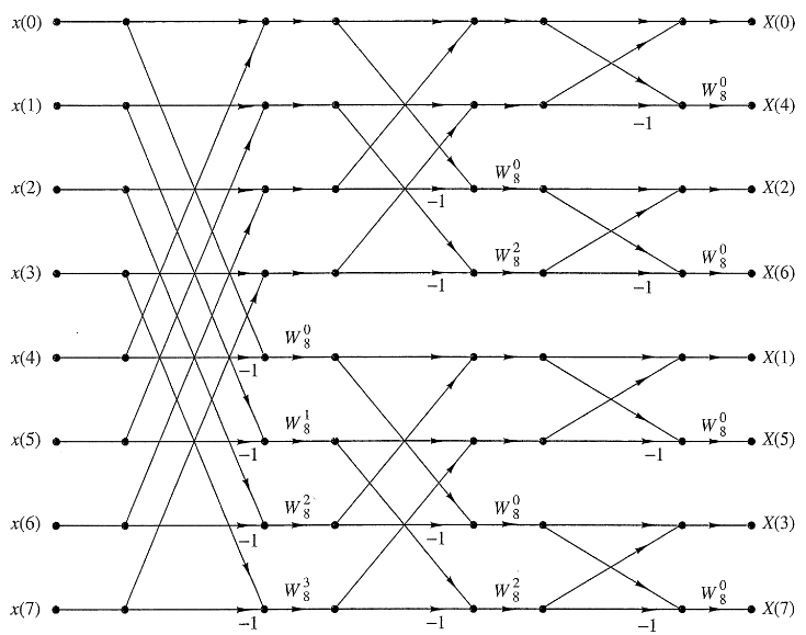
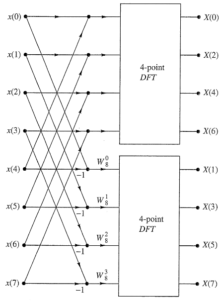
This can futher be observed with a butterfly diagram:

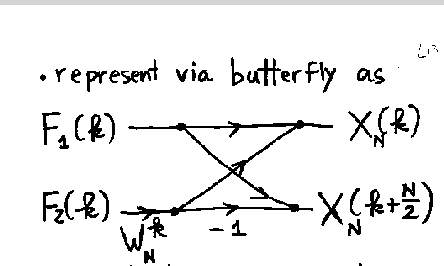
This is the first big computation save that the FFT provides, but it is not nearly all. As can be seen, two non-trivial DFTs are required to be computed.

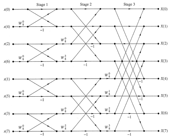
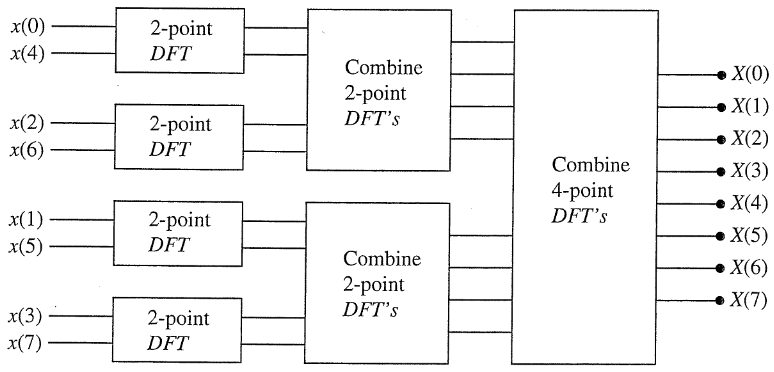
The next step allows us to dramatically improve computational efficiency: we can decimate $f^{(1)}[n]$, $f^{(2)}[n]$ futher until we only compute 2-pt DFTs (only works because $N=2^v$).

In block diagram form:

As can be seen, the ordering of the inputs is a bit interesting. The below figure describes how the ordering maps, from natural to bit-reversed order:

2.1.2. Radix-2 Decimation in Frequency

This is very similar to the decimation in time algorithm.

We start with the DFT:

$$X_N(k)=\sum_{n=0}^{N-1}x[n]e^{-j\frac{2\pi k}{N} n}$$

We wish to split the sum into two halves, as such:

$$X_N(k)=\sum_{n=0}^{N/2-1}x[n]e^{-j\frac{2\pi k}{N} n} + \sum_{n=N/2}^{N-1}x[n]e^{-j\frac{2\pi k}{N} n}$$

Then, we wish to again obtain each sum as a $N/2$-pt DFT:

$$X_N(k)=\sum_{n=0}^{N/2-1}x[n]e^{-j\frac{2\pi k}{N} n} + e^{-j \pi k}\sum_{n=0}^{N/2-1}x[n+\frac{N}{2}]e^{-j\frac{2\pi k}{N} n}$$$$X_N(k)=\sum_{n=0}^{N/2-1}(x[n] + (-1)^kx[n+\frac{N}{2}])e^{-j\frac{2\pi k}{N} n}$$

We now wish to decimate in frequency to obtain the odd and even $k$ values:

$$X_N(2k)=\sum_{n=0}^{N/2-1}(x[n] + x[n+\frac{N}{2}])e^{-j\frac{2\pi k}{N/2} n}$$

$$X_N(2k+1)=\sum_{n=0}^{N/2-1}\{(x[n] - x[n+\frac{N}{2}])e^{-j\frac{2\pi}{N} n}\}e^{-j\frac{2\pi k}{N/2} n}$$

Now let $g^{(1)}[n]=x[n] + x[n+\frac{N}{2}]$ and $g^{(2)}[n]=(x[n] - x[n+\frac{N}{2}])e^{-j\frac{2\pi}{N} n}$. Then

$$\boxed{X_N(2k)=\sum_{n=0}^{N/2-1}g^{(1)}[n]W_{N/2}^{kn}=G_{N/2}^{(1)}(k)}$$

$$\boxed{X_N(2k+1)=\sum_{n=0}^{N/2-1}g^{(2)}[n]W_{N/2}^{kn}=G_{N/2}^{(2)}(k)}$$

In block diagram form:

2.1.3. Efficiency

First, we must decimate $v=log_2(N)$ times. Each decimation involves $N/2$ butterflies, and each butterfly requires 1 multiplication and 2 additions. Therefore, we obtain $\frac{N}{2}log_2(N)$ multiplcations and $Nlog_2(N)$ additions.

Without the FFT algorithm we have $N^2$ multiplcations and $N(N-1)$ additions.

2.2. Divide and Conquer: Non-Prime-pt FFTs

2.2.1. Formulation

Now we move onto the more general case, where $N$ can be factored by two numbers, $M$ and $L$ for $N=ML$. Recall DFT:

$$X_N(k)=\sum_{n=0}^{N-1}x[n]e^{-j\frac{2\pi k}{N}n}$$

We can first decimate in time, as the decimation in time FFT:

$$X_N(k)=\sum_{l=0}^{L-1}\sum_{m=0}^{M-1}x[l+mL]e^{-j\frac{2\pi k}{N}(l+mL)}$$

We can then decimate in frequency, as the decimation in frequency FFT:

$$X_N(q+pM)=\sum_{l=0}^{L-1}\sum_{m=0}^{M-1}x[l+mL]e^{-j\frac{2\pi}{N}(q+pM)(l+mL)}$$

(The order of the above, obviously, does not matter).

Simplifying:

$$e^{-j\frac{2\pi}{N}(q+pM)(l+mL)}=e^{-j\frac{2\pi}{N}ql}e^{-j\frac{2\pi}{M}mq}e^{-j\frac{2\pi}{L}lp}e^{-j 2\pi pm}$$

$$X_N(q+pM)=\sum_{l=0}^{L-1}\{e^{-j\frac{2\pi}{N}ql}[\sum_{m=0}^{M-1}x[l+mL]e^{-j\frac{2\pi}{M}mq}]\}e^{-j\frac{2\pi}{L}lp}$$

In plain english:

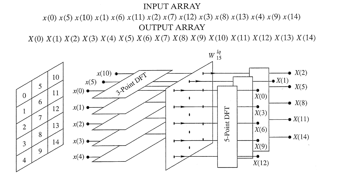
1. Take $L$ $M$-pt DFTs of $x$ decimated at different points according to $x[l+mL]$.
2. Multiply each $M$-pt DFT generated in the previous step by the “twiddle factor” $e^{-j\frac{2\pi}{N}ql}$
3. Take the $L$-pt DFT of the quantity generated in the last step. Do this $M$ times to get all values.

Take the example below of a 15-pt FFT:

2.2.2. Efficiency

Count:

1. $L$ $M$-pt DFTs -> $LM^2$ multiplications.
2. N=ML multiplications by twiddle factor.
3. $M$ $L$-pt DFTs -> $ML^2$ multiplications.

Total:

$$LM^2+ML+ML^2=N(M+L+1) < N^2=N(ML)$$

Because $M+L+1 < ML$.

2.3. Inverse FFT

Recall the DFT and IDFT:

$$X_N(k)=\sum_{n=0}^{N-1}x[n]e^{-j\frac{2\pi k}{N}n}$$

$$x[n]=\frac{1}{N}\sum_{n=0}^{N-1}X_N(k)e^{j\frac{2\pi k}{N}n}$$

Take the conjugate of the IDFT formula:

$$x^*[n]=\frac{1}{N}\sum_{n=0}^{N-1}X_N^*(k)e^{-j\frac{2\pi k}{N}n}$$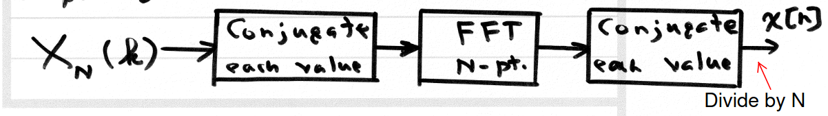

So IFFT is calculated by the FFT.

3. Frequency Domain Sampling / DFT

The basic idea of the DFT is that we are sampling the DTFT of a signal so that we can store it in memory. Recall the DTFT:

$$X(\omega)=DTFT\{x[n]\}=\sum_{n=-\infty}^{\infty}x[n]e^{-j\omega n}$$

We sample $X(\omega)$ as such:

$$X_N(k)=X(\omega_k = \frac{2\pi k}{N})=\sum_{n=0}^{N-1}x[n]e^{-j\frac{2\pi k}{N} n}$$

Which is called the N-point DFT of $x$.

3.1. Various Notes

1. The DFT goes $\omega_k \in [0,2\pi)$

4. Time-Domain Aliasing

4.1. Formulation, Nyquist Sampling

Let

$$X_s(\omega)=X(\omega)\sum_{k=-\infty}^{\infty}\delta(\omega-k\frac{2\pi}{N})$$

Then

$$x_s[n]=x[n]*\sum_{k=-\infty}^{\infty}\frac{N}{2\pi}\delta[n-kN]=\frac{N}{2\pi}\sum_{k=-\infty}^{\infty}x[n-kN]$$

Thus

$$\boxed{x_s[n]=\frac{N}{2\pi}\sum_{k=-\infty}^{\infty}x[n-kN]}$$

Which shows that when we sample in the frequency domain, we get periodic replications of the time domain signal in the time domain.

In order to prevent aliasing, we require

$$\boxed{N>L}$$

Where $L$ is the length of $x$.

5. DFT-Based Processing

The advantage of DFT-based processing over simple convolution between filters is that the FFT makes DFT computation much more efficient than convolution. However, you must be careful about time-domain aliasing.

5.1. Time-Domain Aliasing

Let’s assume you have a signal $x$ of length $L$ and you want to pass it through a digital filter $h$ of length $M$. The result will be a signal $y$ of length $L+M-1$.

Let $M < L < N < L+M-1$.

You may think $Y_N(k)=X_N(k)H_N(k)$ will return the same signal $y[n]=x[n]*h[n]$ when you compute the IFFT, but this is not what happens, since $N < L + M - 1$, the signal is acutally an aliased. Instead, some signal $y_p$ is returned.

This signal obeys the following formula:

$$y_p[n]=\sum_{l=-\infty}^{\infty}y[n-lN]\{u[n]-u[n-N]\}$$

Or, alternatively $y_p$ is the result of circular convolution, not linear convolution, between $x$ and $h$.