The purpose of this week is to analyze perfect reconstruction filter banks (PRFBs) of size $M=2^v$.

1. Application

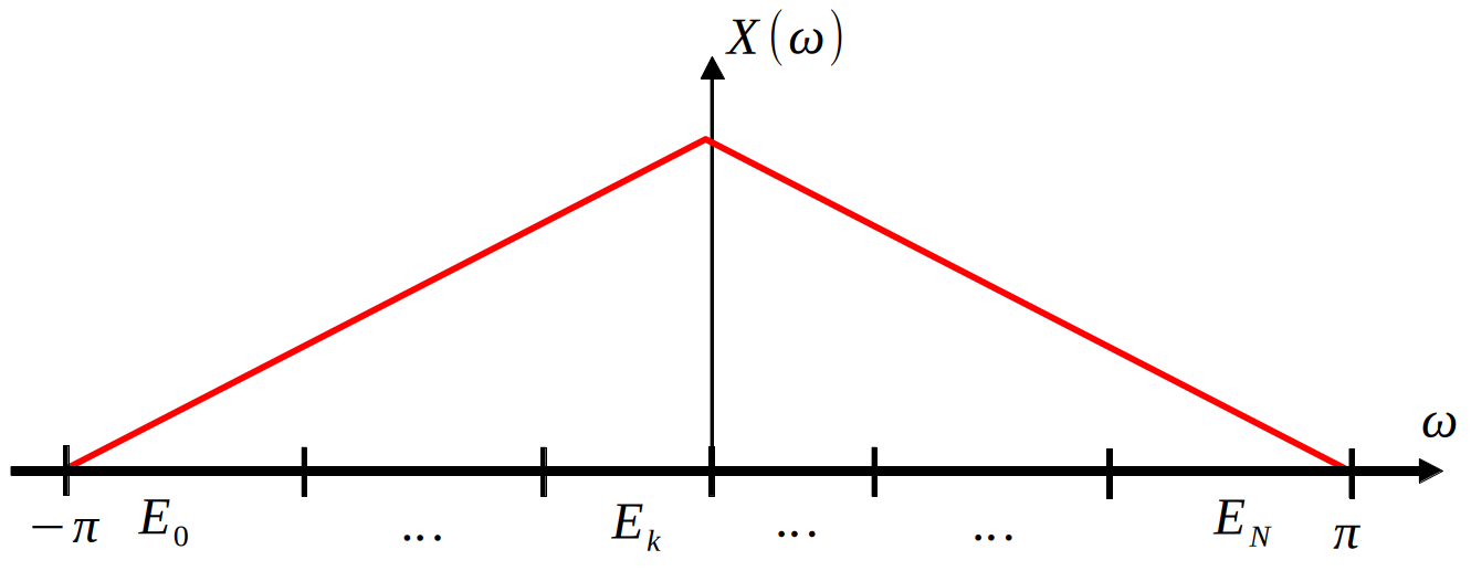
The primary application considered here is subband coding for audio compression. In this application, the spectrum of a signal is split up into $N+1$ chunks. Each chunk is then assigned a number of bits according to the energy contained in that chunk $E_k$ and a function that relates that energy to the response in the human ear.

PRFBs allow us to split a signal into different subbands to manipulate each subband as we please. They get their name from the fact that, if nothing is done to each subband, the system is able to perfectly reconstruct the input at the output.

2. 2-Channel PRFB

The most basic PRFB case is studied to understand the more general formulations.

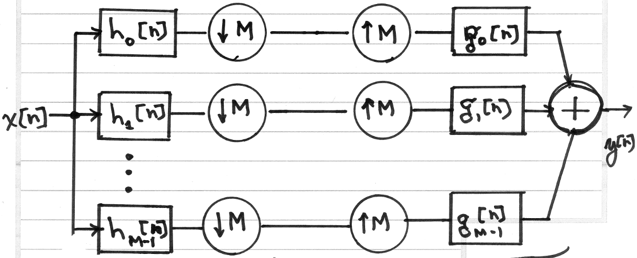
The left-hand side of the diagram is called the analysis side, and the right-hand side of the diagram is called the synthesis side. For now, let the filters on the analysis side be $h_0$ and $h_1$, and the filters on the synthesis side be $g_0$ and $g_1$.

2.1. Basic Analysis

Using the decimation formula obtained in week 8, we obtain:

$$Z_0(\omega) = \frac{1}{2}H_0(\frac{\omega}{2})X(\frac{\omega}{2})+\frac{1}{2}H_0(\frac{\omega-2\pi}{2})X(\frac{\omega-2\pi}{2})$$

$$Z_1(\omega) = \frac{1}{2}H_1(\frac{\omega}{2})X(\frac{\omega}{2})+\frac{1}{2}H_1(\frac{\omega-2\pi}{2})X(\frac{\omega-2\pi}{2})$$

Now using the interpolation formula obtained in week 8, we obtain:

$$V_0(\omega) = Z_0(2\omega) = \frac{1}{2}H_0(\omega)X(\omega)+\frac{1}{2}H_0(\omega-\frac{2\pi}{2})X(\omega-\frac{2\pi}{2})$$

$$V_1(\omega) = Z_1(2\omega) = \frac{1}{2}H_1(\omega)X(\omega)+\frac{1}{2}H_1(\omega-\frac{2\pi}{2})X(\omega-\frac{2\pi}{2})$$

Continuing:

$$Y_0(\omega) = V_0(\omega)G_0(\omega) = \frac{1}{2}H_0(\omega)G_0(\omega)X(\omega)+\frac{1}{2}G_0(\omega)H_0(\omega-\pi)X(\omega-\pi)$$

$$Y_1(\omega) = V_1(\omega)G_1(\omega) = \frac{1}{2}H_1(\omega)G_1(\omega)X(\omega)+\frac{1}{2}G_1(\omega)H_1(\omega-\pi)X(\omega-\pi)$$

Continuing:

$$Y(\omega)=Y_0(\omega)+Y_1(\omega)= \frac{1}{2}H_0(\omega)G_0(\omega)X(\omega)+\frac{1}{2}G_0(\omega)H_0(\omega-\pi)X(\omega-\pi) + \frac{1}{2}H_1(\omega)G_1(\omega)X(\omega)+\frac{1}{2}G_1(\omega)H_1(\omega-\pi)X(\omega-\pi) $$

Simplifying to group by $X$,

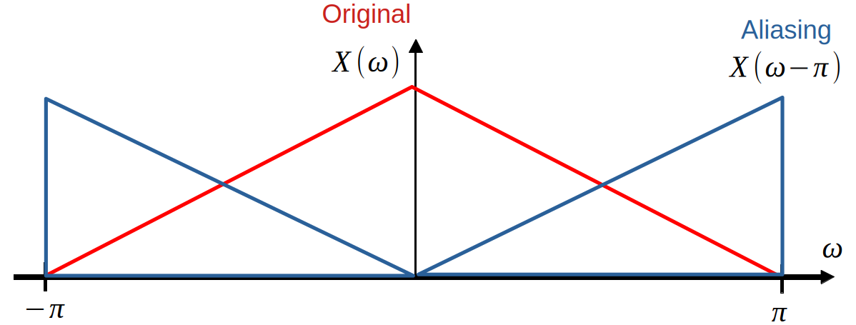
$$\boxed{Y(\omega)=\frac{1}{2}\{H_0(\omega)G_0(\omega)+H_1(\omega)G_1(\omega)\}X(\omega) + \frac{1}{2}\{G_0(\omega)H_0(\omega-\pi)+G_1(\omega)H_1(\omega-\pi)\}X(\omega-\pi)}$$

As can be seen, $Y(\omega)$ contains two terms, one involving the original signal $X(\omega)$ and another involving an aliasing term, $X(\omega-\pi)$.

2.2. Conditions for Perfect Reconstruction

To achieve perfect reconstruction, we require

$$Y(\omega)=cX(\omega)$$

Where $c$ is a complex constant. This corresponds to

$$y[n]=Cx[n-n_c]$$

In the time domain, which means $y$ is a shifted/scaled version of $x$.

From the analysis above, we require the below two conditions in order to satisfy this condition:

1. Alias-free: $$\boxed{G_0(\omega)H_0(\omega-\pi)+G_1(\omega)H_1(\omega-\pi) = 0}$$
2. Distortionless: $$\boxed{H_0(\omega)G_0(\omega)+H_1(\omega)G_1(\omega)=c}$$

2.3. Example

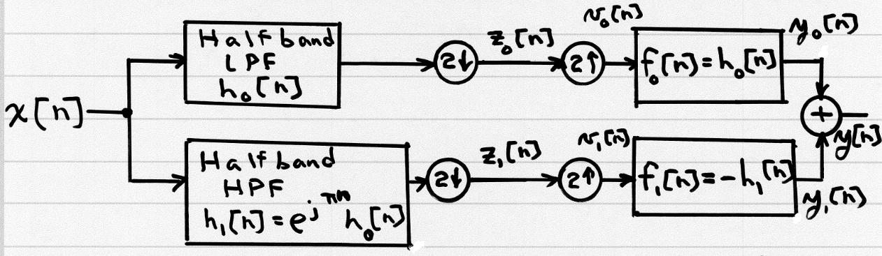
In the case where the filters are the ones given in the above diagram, where $H_0(\omega)$ is a low-pass filter,

$$H_1(\omega)=H_0(\omega-\pi)$$

$$G_0(\omega)=H_0(\omega)$$

$$G_1(\omega)=-H_0(\omega-\pi)$$

So we have

1. Alias-free: $$H_0(\omega)H_0(\omega-\pi)-H_0(\omega-\pi)H_0(\omega) = 0 = 0$$ So with these choices, we guarantee alias-free.
2. Distortionless: $$H_0(\omega)H_0(\omega)-H_0(\omega-\pi)H_0(\omega-\pi)=H_0(\omega)^2-H_0(\omega-\pi)^2=c$$

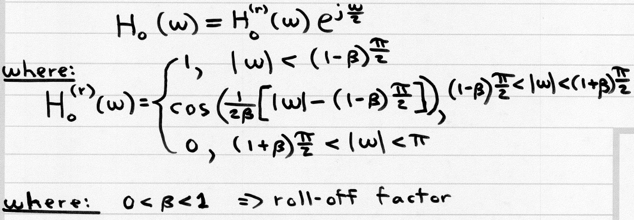
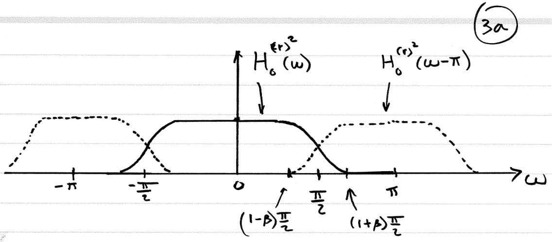
Therefore, we must choose $H_0(\omega)$ so that the distortionless condition:

$$H_0(\omega)^2-H_0(\omega-\pi)^2=c$$

is met. An example of such a filter is the raised-root cosine filter.

3. Extension to Powers of 2

The extension to powers of two rests on the concept of the tree-structure. The idea is to first pass the signal through a 2-ch PRFB, and take the resulting signal and pass that through another 2-ch PRFB. This will split the spectrum in a binary-search way, achieving our desired effect. The below figures show the tree structure for the 8($2^3$)-channel case.

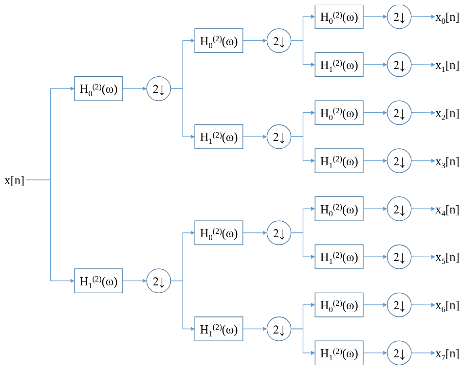
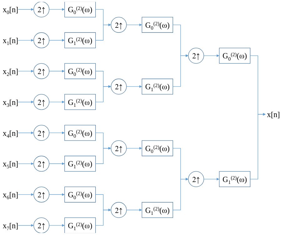
As long as the conditions found in the previous section hold for $H_0^{(2)}(\omega)$, $H_1^{(2)}(\omega)$, $G_0^{(2)}(\omega)$ and $G_1^{(2)}(\omega)$, perfect reconstruction is achieved.

3.1. The Noble Identities

The noble identities allow us to make a much more efficient implementation of the tree-structure PRFB.

3.2. Extension Process