ECE552 Final Notes
A summary of topics on the final exam for ECE 552.
- Atomic Radiation
- Laser Amplification and Oscillation
0. Preamble: Units
- 1 Angstrom = $10^{-10}m$
- Plancks constant = $6.62607015×10^{-34} J⋅Hz^{-1}$
- Speed of light = $2998\cdot 10^{10} \frac{m}{s}$
- 1 electron volt = charge of an electron = $1.602176634×10^{-19}C$
- characteristic impedance of free space $\eta_0$ = $120\pi \Omega$
- 1 amu = $1.660539\cdot10^{-24}$ grams
- Boltzmann constant: $1.380649\cdot10^{−23} J⋅K^{−1}$
1. Atomic Radiation (Chapter 7)
1.1 Einstein Approach
The following applies for broadband light, e.g. light incoming on an atomic system whose frequency domain width is much larger than the spectral line shape’s. See general equation in section 1.2.
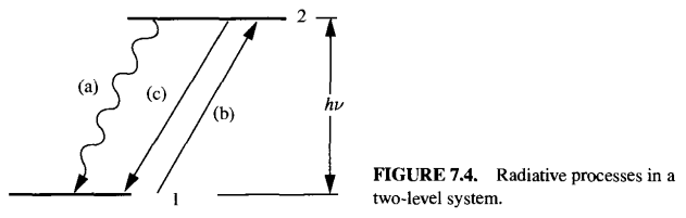
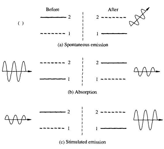
1.1.1 Spontaneous Emission (SpE)
$$\frac{dN_2}{dt}|_{spontaneous\ emission}=-A_{21}N_2$$1.1.2 Absoroption (Ab)
$$\frac{dN_2}{dt}|_{absoprtion}=B_{12}N_1\rho(\nu)$$1.1.3 Sitmulated Emission (StE)
$$\frac{dN_2}{dt}|_{stimulated\ emission}=-B_{21}N_2\rho(\nu)$$Adds a photon:
- At the same frequency
- In the same polarization
- In the same direction
- In the same phase of the stimulating wave.
1.1.4 Relationship Between the Coefficients
$$\frac{dN_2}{dt}|_{radiative}=-A_{21}N_2+B_{12}N_1\rho(\nu)-B_{21}N_2\rho(\nu)$$At equilibrium, it can be shown that:
$$g_2B_{21}=g_1B_{12}$$Where $g_i$ is the number of ways that an atom can have energy $E_i$. This is related to the total angular momentum $J_i$ by
$$g_i=2J_i+1$$Through the same method it is also shown that
$$\frac{A_{21}}{B_{21}}=\frac{8\pi n^2 n_g^2 h \nu^3}{c^3}$$By solving for $\rho(\nu)$ and comparing to Planck’s blackbody result:
$$\rho(\nu)=(\frac{8\pi n^2 n_g^2 h \nu^3}{c^3})\cdot h\nu \cdot \frac{1}{e^{\frac{h\nu}{kT}}-1}$$- $\rho(\nu)$ : energy density
- $A_{21}$ : spontaneous emission rate
- $B_{12}$ : absorption rate
- $B_{21}$ : stimulated emission rate
1.2 Line Shape
By the uncertainty principle, each energy level must actually consist of a narrow band of frequencies around the center frequency of the level.
1.2.1 Definition
$g(\nu)d\nu$ : the probability that a spontaneously emitted photon will appear at a frequency between $\nu$ and $\nu + d\nu$. Therefore:
$$\int_{0}^{\infty}g(\nu)d\nu=1$$1.2.2 Updated Radiative Rate Equation
In the case where $\rho(\nu)$ has a much smaller bandwidth than $g(\nu)$, we must account for the fact that only a certain fraction of the energies available in an energy state will be stimulated by the incoming light. Therefore we modify the radiative rate equations as follows:
$$\frac{dN_2}{dt}|_{radiative}=-A_{21}N_2[\int_{0}^{\infty}g(\nu')d\nu'=1]+B_{12}N_1[\int_{0}^{\infty}\rho(\nu')g(\nu')d\nu']-B_{21}N_2[\int_{0}^{\infty}\rho(\nu')g(\nu')d\nu']$$However, we wish to analyze the case where
$$\rho(\nu')\approx \rho_{\nu}\delta(\nu'-\nu)$$So we have the opposite extreme case from the original einstein equations, which yields:
$$\frac{dN_2}{dt}|_{radiative}=-A_{21}N_2+B_{12}N_1\rho_{\nu}g(\nu)-B_{21}N_2\rho_{\nu}g(\nu)$$We now wish to rewrite the original equations with the following substitutions:
$$B_{12}=\frac{g_2}{g_1}B_{21}$$$$B_{21}=\frac{c^3}{8\pi n^2 n_g^2 h \nu^3}A_{21}=\frac{c}{n_g}\cdot \frac{\lambda_0^2}{8\pi n^2}\cdot \frac{A_{21}}{h\nu}$$$$\rho_{\nu}=\frac{I_{\nu}}{c/n_g}$$and define the stimulated emission cross section:
$$\boxed{\sigma_{StE}(\nu)=A_{21}\frac{\lambda^2}{8\pi n^2}g(\nu)}$$We obtain
$$\boxed{\frac{dN_2}{dt}|_{radiative}=-A_{21}N_2-\frac{\sigma_{StE}(\nu)I_{\nu}}{h\nu}[N_2-\frac{g_2}{g_1}N_1]}$$1.3 Amplification
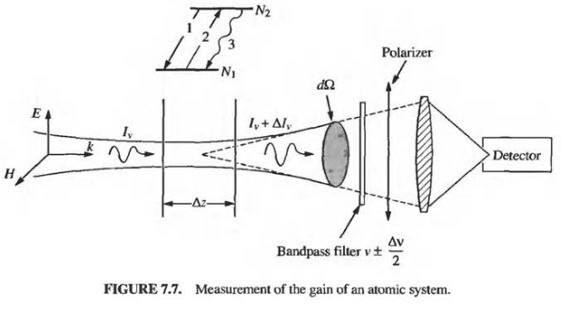
With the above setup and proper accounting, it can be found that:
$$\boxed{\frac{dI_{\nu}}{dz}=[A_{21}\frac{\lambda^2}{8\pi n^2}g(\nu)][N_2-\frac{g_2}{g_1}N_1]I_{\nu}=\gamma(\nu)I_{\nu}}$$With
$$\gamma(\nu)=[A_{21}\frac{\lambda^2}{8\pi n^2}g(\nu)][N_2-\frac{g_2}{g_1}N_1]=\sigma_{StE}(\nu)N$$Where $N=N_2-\frac{g_2}{g_1}N_1$ is the population inversion.
Therefore the condition for gain is:
$$\boxed{N_2>\frac{g_2}{g_1}N_1}$$1.3.1 Small Signal Gain
If the intensity doesn’t change the population densities, $N_1$ and $N_2$, then $\gamma(\nu) \rightarrow \gamma_0(\nu)$, which is called the small signal gain. If it is a small signal:
$$I(z)=e^{\gamma_0(\nu)z}$$1.3.2 Cross Sections
The gain DE can be re-written as
$$\frac{dI_{\nu}}{dz}=[A_{21}\frac{\lambda^2}{8\pi n^2}g(\nu)][N_2-\frac{g_2}{g_1}N_1]I_{\nu}=(\sigma_{StE}(\nu)N_2-\sigma_{Ab}(\nu)N_1)I_{\nu}$$So that
$$\gamma(\nu)=(\sigma_{StE}(\nu)N_2-\sigma_{Ab}(\nu)N_1)$$1.4 Broadening
1.4.1 Homoheneous Broadening
$$g(\nu)=\frac{\Delta \nu}{2\pi [(\nu_0-\nu)^2+(\Delta\nu/2)^2]}$$Where
$$\Delta\nu=\frac{1}{2\pi}\{\frac{1}{\tau_2}+\frac{1}{\tau_1}\}=\frac{1}{2\pi}\{(A_2+k_2)+(A_1+k_1)\}$$Where $k$ represents general losses. When there are no such losses:
$$\frac{1}{\tau_2}=\sum_{j<2}A_{2j}$$The branching ratio is
$$\phi_{21}=\frac{rate\ of\ decay\ from\ states\ 2\ to\ 1}{sum\ of\ all\ decay\ rates\ from\ state\ 2}=\frac{A_{21}}{\sum_{j<2}A_{2j}+k_2}$$Lifetime broadening is the theoretical minimum and is often drowned out by larger broadening due to other mechanisms, so it is not too important.
1.4.2 Collisional Broadening
The fundamental mechanism here is that elastic collisions between atomic systems lead to a discontinuous change in the phase of radiation, which leads to broadening in the frequency domain.
$$\Delta\nu=\frac{1}{2\pi}\{(A_2+k_2)+(A_1+k_1)+2\nu_{col}\}$$$$\nu_{col}=N_m \sigma[\frac{8kT}{\pi}(\frac{1}{M_m}+\frac{1}{M_n})]^{1/2}$$1.4.3 Inhomogeneous/Doppler Broadening
$$\Delta\nu_D=(\frac{8kTln(2)}{Mc^2})^{1/2}\nu_0$$$$g(\nu)=(\frac{4ln(2)}{\pi})^{1/2}\frac{1}{\Delta\nu_D}exp[-4ln(2)(\frac{\nu-\nu_0}{\Delta\nu_D})]$$2. Laser Amplification and Oscillation (Chapter 8)
2.1 Homogeneous Broadened Transition
2.1.1 Amplification and Oscillation
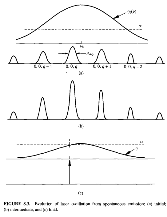
The above figure gives an idea of the evolution of a laser’s gain.
- Obtain population inversion with pump.
- Spontaneous emission releases energy into all of the many available modes and directions.
- The cavity selects those modes and directions that achieve resonance.
- Intensity of the cavity modes increases and more stimulated emission occurs.
- The rate of stimulated emission reaches the rate of pumping, saturating population inversion. This is what is explored in the next section, gain saturation.
Some details:
- The gain coefficient has saturated to the loss coefficient at the frequency of laser operation (aka the cavity mode).
- All modes but the dominant one are now below losses.
- Therefore laser oscillation occurs at the dominant cavity mode.
2.1.2 Gain Saturation
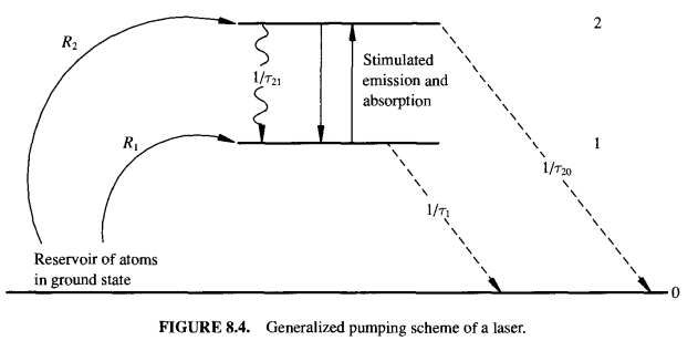
The dynamics of the above system is given by the following:
$$\frac{dN_2}{dt}=R_2-\frac{N_2}{\tau_2}-\frac{I_{\nu}}{h\nu}(\sigma_{StE}(\nu)N_2-\sigma_{Ab}(\nu)N_1)$$$$\frac{dN_1}{dt}=R_1+\frac{N_2}{\tau_{21}}-\frac{N_1}{\tau_1}+\frac{I_{\nu}}{h\nu}(\sigma_{StE}(\nu)N_2-\sigma_{Ab}(\nu)N_1)$$Let $\sigma_{StE}=\sigma_{Ab}=\sigma$
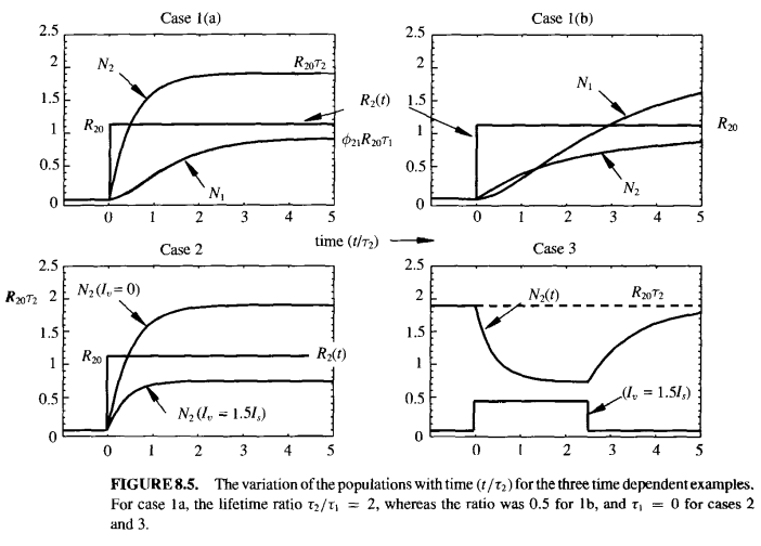
2.1.2.a Case 1: No incoming light
Assume $I_{\nu}=0$, $R_1=0$, and $R_2$ is a step function / constant. Then:
$$\frac{dN_2}{dt}=R_2-\frac{N_2}{\tau_2}$$$$\frac{dN_1}{dt}=R_1+\frac{N_2}{\tau_{21}}-\frac{N_1}{\tau_1}$$These can be solved with the tools of elementary differential equations. Solutions to homeworks 4 and 5 can be examined for more details.
$$N_2(t)=R_2\tau_2(1-e^{-t/\tau_2})$$$$N_1(t)=\phi_{21}R_2\tau_1\{1+\frac{\tau_1/\tau_2}{1-\tau_1/\tau_2}e^{-t/\tau_1}-\frac{1}{1-\tau_1/\tau_2}e^{-t/\tau_2}\}$$2.1.2.b Case 2: Best Laser Action
The conditions for best lasing action are:
- $\tau_1<<\tau_2$ : empty $N_1$ quicker than $N_2$
- $R_1 << R_2$ : pump $N_2$ much more than $N_1$
Assume $\tau_1=0$ (just to simplify the math). Actually a good model for excimer lasers and Nd:YAG. Therefore:
$$N_1(t)=0$$so
$$\frac{dN_2}{dt}=R_2-\frac{N_2}{\tau_2}-\frac{I_{\nu}}{h\nu}\sigma(\nu)N_2$$The solution is
$$N_2(t)=\frac{R_2\tau_2}{1+I_{\nu}/I_s}\{1-exp[-\frac{t}{\tau_2}(1+\frac{I_{\nu}}{I_s})]\}$$Where the saturation intensity for this case is:
$$I_s=\frac{h\nu}{\sigma\tau_2}$$This is explored further below in case 4.
Independent of the above, we also prefer the following for optimal lasing:
- $\tau^{-1}_{20}<<\tau^{-1}_{21}$ : maximize energy utility by operating in the lasing transition (2->0 takes away from lasing transition)
2.1.2.c Case 3: Light Pulse
Assume $\tau_1=0$ (just to simplify the math again).
$$N_1(t)=0$$so
$$\frac{dN_2}{dt}=R_2-\frac{N_2}{\tau_2}-\frac{I_{\nu}}{h\nu}\sigma(\nu)N_2$$$$N_2(t)=\frac{R_2\tau_2}{1+I_{\nu}/I_s}\{(I_{\nu}/I_s)exp[-\frac{t}{\tau_2}(1+I_0/I_s)]+1\}$$2.1.2.d Case 4: Steady State (actual saturation!!!)
As discussed above, the dominant cavity mode is the only we evaluate around the resonance frequency $\nu_0$
$$\frac{dN_2}{dt}=0=R_2-\frac{N_2}{\tau_2}-\frac{I_{\nu}}{h\nu}(\sigma_{StE}(\nu)N_2-\sigma_{Ab}(\nu)N_1)$$$$\frac{dN_1}{dt}=0=R_1+\frac{N_2}{\tau_{21}}-\frac{N_1}{\tau_1}+\frac{I_{\nu}}{h\nu}(\sigma_{StE}(\nu)N_2-\sigma_{Ab}(\nu)N_1)$$Through lots of math, we obtain $\gamma(\nu)=(N_2-N_1)\sigma$.
$$\gamma(\nu)=\frac{[R_2\tau_2(1-\frac{\tau_1}{\tau_{21}})-R_1\tau_1]\sigma(\nu)}{1+(\tau_1+\tau_2-\frac{\tau_1\tau_2}{\tau_{21}})\sigma(\nu)\frac{I_{\nu}}{h\nu}}$$If $I_{\nu}$ is small enough so that the denominator is approximately 1,
$$\boxed{\gamma_0(\nu)=[R_2\tau_2(1-\frac{\tau_1}{\tau_{21}})-R_1\tau_1]\sigma(\nu)}$$Also define $I_s$ to be:
$$\boxed{I_s=\frac{h\nu}{\sigma(\nu)\tau_2}\frac{1}{1+\frac{\tau_1}{\tau_2}(1-\frac{\tau_2}{\tau_{21}})}}$$With
$$\sigma(\nu)=\sigma(\nu_0)\bar{g}(\nu)$$Where
$$\bar{g}(\nu)=\frac{(\Delta\nu/2)^2}{(\nu-\nu_0)^2+(\Delta\nu/2)^2}$$Since we are assuming resonance ($\bar{g}$ is peak-normalized line shape).
Thus $\gamma(\nu)$ can be written as:
$$\boxed{\gamma(\nu,I_{\nu})=\frac{1}{I_{\nu}}\frac{dI_{\nu}}{dz}=\frac{\gamma_0(\nu)}{1+\frac{I_{\nu}}{I_s}}}$$Solving for $I_{\nu}$ with separation of variables:
$$\boxed{ln(G)+\bar{g}(\nu)\frac{I_{\nu}(0)}{I_s}[G-1]=\gamma_0(\nu)d}$$In the small signal case, ($GI_{\nu}(0) << I_s$ and $I_{\nu}(0) << I_s$) this reduces to
$$G_0(\nu)=e^{\gamma_0(\nu)d}$$In the limit as the input intensity goes to infinity, this reduces to
$$\frac{\bar{g}(\nu)I_{\nu}(0)}{I_s}[G-1]=\gamma_0(\nu)d$$In terms of extracted power,
$$GI_{\nu}(0)\bar{g}(\nu)-I_{\nu}(0)\bar{g}(\nu)=\Delta I_{\nu}=\gamma_0 d I_s$$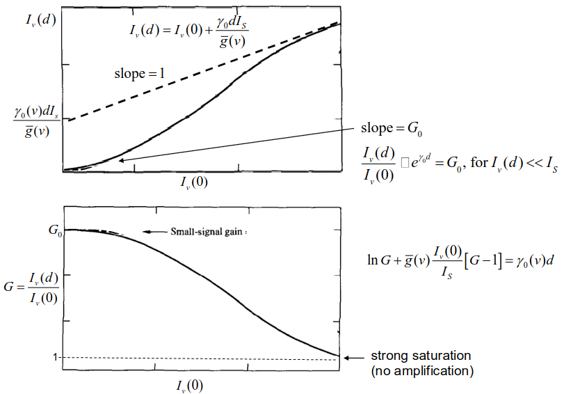
2.2 Inhomogeneous Broadened Transition
2.2.1 Amplification and Oscillation
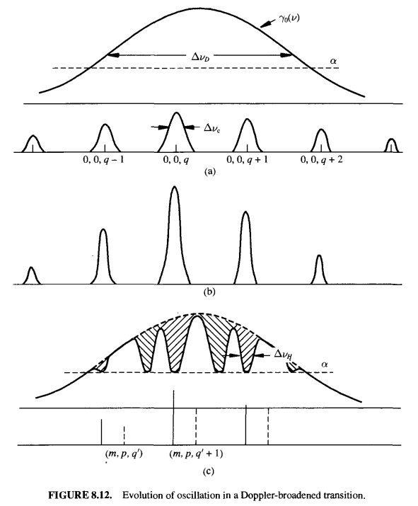
The above figure gives an idea of the evolution of a laser’s gain in an inhomogeneous system
2.2.2 Gain Saturation
2.3 Amplified Spontaneous Emission (ASE)
When spontaneous emission is amplified, it:
- limits the gain of an amplifier
- creates broad-band radiation
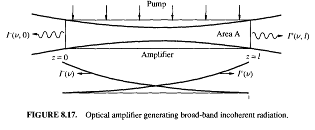
Setting up IVP:
$$\frac{dI^+(\nu,z)}{dz}=\gamma_0(\nu)I^+(\nu,z)+spont.\ noise$$$$\frac{d}{dz}[I^+(\nu,z)d\nu]=\gamma_0(\nu)I^+(\nu,z)+h\nu A_{21}N_2g(\nu)d\nu\frac{d\Omega}{4\pi}$$$$I^+(\nu,0)=0$$Solution:
$$I^+(\nu,l)=\frac{h\nu A_{21}N_2g(\nu)}{\gamma_0(\nu)}[exp(\gamma_0(\nu)l)-1]\frac{d\Omega}{4\pi}$$But since
$$G_0(\nu)=exp(\gamma_0(\nu)l)$$and
$$\gamma(\nu)=[A_{21}\frac{\lambda^2}{8\pi n^2}g(\nu)][N_2-\frac{g_2}{g_1}N_1]=\sigma_{StE}(\nu)N$$We have
$$\boxed{I^+(\nu,l)=\frac{8\pi h\nu^3 n^2}{c^2}\frac{N_2}{N}[G_0(\nu)-1]\frac{d\Omega}{4\pi}}$$2.3.1 Case 1: Optically Thin Medium
Assume
$$G_0(\nu)-1\approx \gamma_0(\nu)l$$We then have:
$$I^+(\nu,l)=h\nu A_{21}N_2g(\nu)l\frac{d\Omega}{4\pi}=h\nu A_{21}N_2g(\nu)l\frac{d\Omega}{4\pi}\frac{V}{A}$$Note that there is no amplification, just random emission along the length.
2.3.2 Case 2: Thermal Population
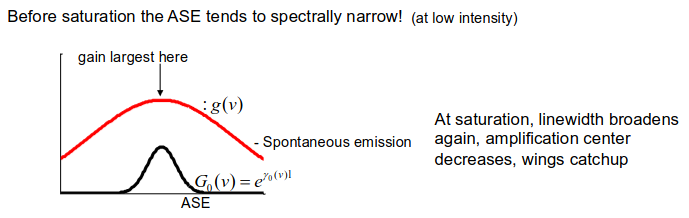
$$I^+(\nu,l)=\frac{8\pi h\nu^3}{c^2}\frac{1}{1-exp(h\nu/kT)-1}[1-exp(-|\gamma_0(\nu)|l)]\frac{d\Omega}{4\pi}$$2.3.3 Spectral Narrowing by ASE
2.3.4 ASE Gain Saturation
Assume:
$$g(\nu)\Delta\nu \approx 1$$$$\tau_2A_{21}\approx 1$$
$$N_2 >> N_1$$$$\boxed{G_{0_{max}}(\nu_0)\approx 1+\frac{4\pi l^2}{A}}$$
Limits small signal gain only, not energy extraction.
2.4 A Different Viewpoint of Laser Oscillation
2.4.1 Photon Population
- $A_{21}NV$ - rate of generation for spontaneous emission. Modes are separated by $\Delta\nu=\frac{c}{2nd}$
- $g(\nu)\Delta\nu=g(\nu)[\frac{c}{2nd}]$ - fraction of emission that appears in $\Delta\nu$
- There are $\frac{8\pi n^3\nu^2}{c^3}V\cdot\Delta\nu$ modes in the volume, but only the $TEM_{0,0,q}$ mode has high Q.
Spontaneous emission:
$$\frac{dN_p}{dt}|_{spont.}=(1)(2)/(3)=N_2c[A_{21}\frac{\lambda^2}{8\pi}g(\nu)]=N_2c\sigma_{SE}$$Cavities with gain:
$$\frac{dN_p}{dt}|_{cavity\ with\ gain}=\frac{G^2R_2R_1-1}{2nd/c}N_p$$Therefore
$$\frac{dN_p}{dt}=\frac{G^2R_2R_1-1}{2nd/c}N_p+N_2c\sigma_{SE}$$(1) $N_p~0$
$N_p$ incerases but output is very small
(2) $N_p$ large
$$N_p(t)=N_p(0)exp[\frac{G^2R_1R_2-1}{2nd/c}t]$$2.4.2 Gain Saturation
In the steady state,
$$\boxed{(1-G^2R_1R_2)=\frac{h\nu}{P_{out}}(1-R_1R_2)N_2^{(S)}c\sigma_{Ste}}\approx10^{-7}$$(recalling $\frac{P_{out}}{h\nu}=\frac{N_p}{2nd/c}(1-R_1R_2)$)
2.4.3 Minimum Laser Linewidth
Schawlow-Townes:
$$\boxed{\Delta\nu_{osc}=2\pi \frac{h\nu}{P_{out}}(1-\frac{g_2N_1^{(S)}}{g_1N_2^{(S)}})^{-1}(\Delta\nu_{1/2})^{1/2}}$$$\Delta\nu_{1/2}=\frac{1}{2\pi\tau_p}=\frac{c}{2\pi d}(1-R_1R_2)$
6. Homework
6.1 Homework 4
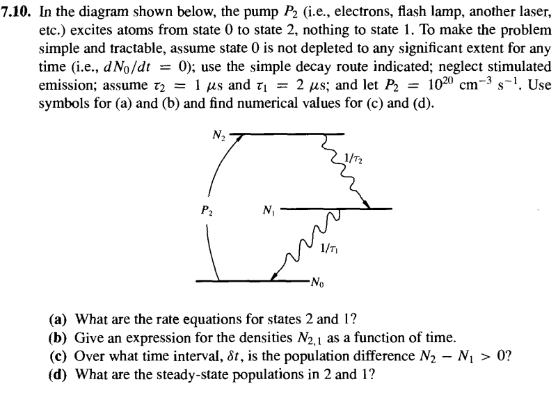
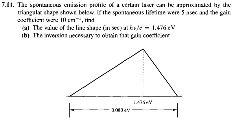
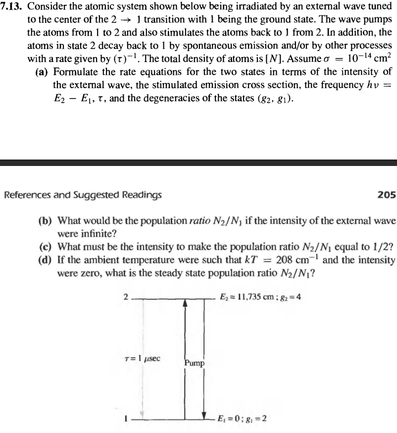
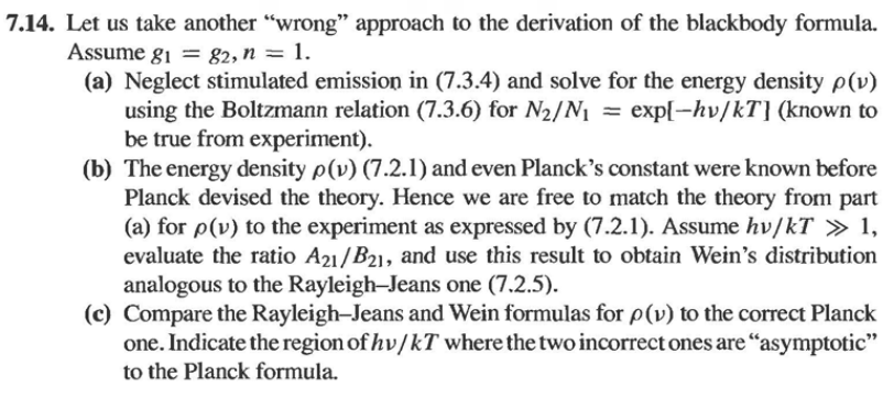
7.6, 7.10, 7.11, 7.13, 7.14
6.1.1 Problem 1

6.1.2 Problem 2
6.1.3 Problem 3
6.1.4 Problem 4
6.1.5 Problem 5
6.2 Homework 5
8.1, 8.2, 8.4, 8.17, 8.27
6.2.1 Problem 1
Solution:
(a)
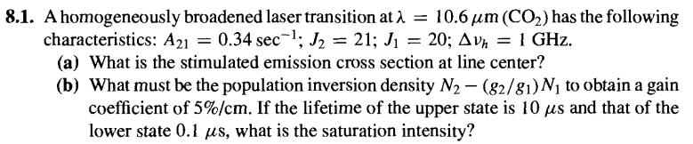
$$\sigma_{StE}(\nu_0)=A_{21}\frac{\lambda^2}{8\pi n^2}g(\nu_0)$$$$g(\nu_0)=\frac{\Delta\nu}{2\pi[(\nu_0-\nu_0)^2+(\Delta\nu/2)^2]}=\frac{2}{\pi\Delta\nu}$$
$$\boxed{\sigma_{StE}(\nu_0)=A_{21}\frac{\lambda^2}{4\pi^2n^2\Delta\nu}}$$
All variables are known (assume $n=1$)
The result comes out to $9.68\cdot 10^{-18} cm^2$
(b)
$$\gamma(\nu)=\sigma_{StE}(\nu)N \Rightarrow N = \frac{\gamma_{des}}{\sigma_{StE}}\approx 5.17 \cdot 10^{15} cm^{-3}$$Thus the first part is completed.
In general, the saturation intensity is found as:
$$I_s=\frac{h\nu}{\sigma(\nu)\tau_2}\frac{1}{1+\frac{\tau_1}{\tau_2}(1-\frac{\tau_2}{\tau_{21}})}$$Since $\tau_1 << \tau_2$, $I_s$ can be approximated as
$$I_s \approx \frac{h\nu}{\sigma(\nu)\tau_2} = \frac{hc}{\lambda\sigma(\nu)\tau_2} \approx 193.5 W/cm^2$$Thus the problem is completed.
6.2.2 Problem 2
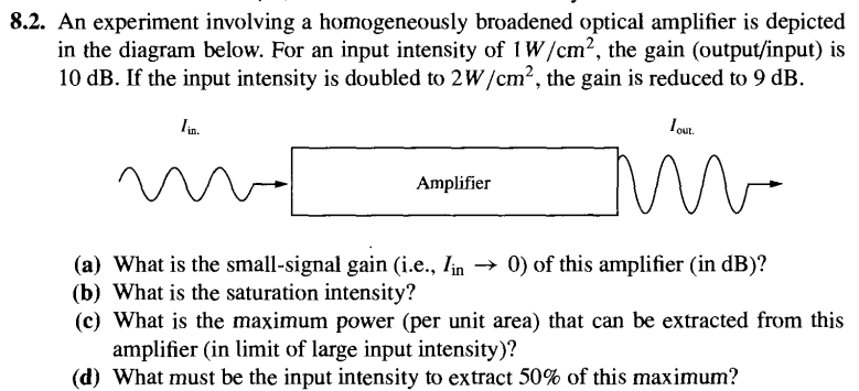
Solution:
(a,b)
$$ln(G_1)+\frac{I_1(0)}{I_s}[G_1-1]=\gamma_0 d=ln(G_0)$$$$ln(G_2)+\frac{I_2(0)}{I_s}[G_2-1]=\gamma_0 d=ln(G_0)$$
Subtract the two equations:
$$ln(G_1/G_2)+\frac{1}{I_s}\{I_1(0)[G_1-1]-I_2(0)[G_2-1]\}=0$$$$I_s=\frac{I_2(0)[G_2-1]-I_1(0)[G_1-1]}{ln(G_1/G_2)}\approx 22.4 W/cm^2$$Substitute solution back into either of the first two equations to obtain
$$G_0=e^{\gamma_0d}\approx 14.94\approx11.74dB$$(c)
$$\Delta I_{\nu}=\gamma_0 d I_s\approx 60.6 W/cm^2$$(d)
$$I_{\nu}(d)-I_{\nu}(0)=0.5\Delta I_{\nu}$$$$ln(\frac{I_{\nu}(d)}{I_{\nu}(0)})+\frac{I_{\nu}(d)-I_{\nu}(0)}{I_s}=\gamma_0 d$$So
$$ln(\frac{\Delta I_{\nu}+I_0}{I_{\nu}(0)})+\frac{0.5\Delta I_{\nu}}{I_s}=\gamma_0 d$$$$I_{\nu}(0)\approx10.6W/cm^2$$6.2.3 Problem 3
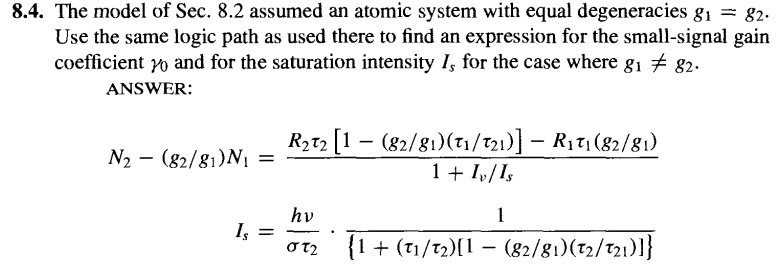
Solution:
$$\sigma_{Ab}=\sigma_{Ste}\frac{g_2}{g_1}$$$$\frac{dN_2}{dt}=R_2-\frac{N_2}{\tau_2}-\frac{\sigma I_{\nu}}{h\nu}N_2+\frac{g_2}{g_1}\frac{\sigma I_{\nu}}{h\nu}N_1$$$$\frac{dN_2}{dt}=R_1-\frac{N_1}{\tau_1}+\frac{N_2}{\tau_{21}}+\frac{\sigma I_{\nu}}{h\nu}N_2-\frac{g_2}{g_1}\frac{\sigma I_{\nu}}{h\nu}N_1$$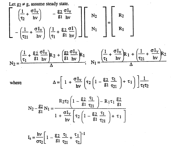
6.2.4 Problem 4
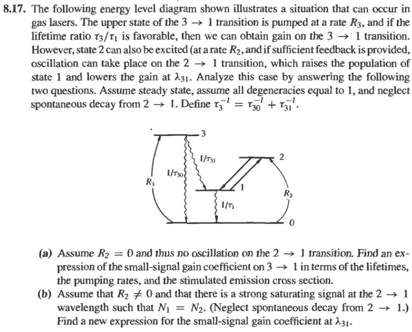
Solution:
(a)
Diff eq:
(assume equal degeneracies)
$$\frac{dN_3}{dt}=R_3-\frac{N_3}{\tau_3}=0$$$$\frac{dN_1}{dt}=\frac{N_3}{\tau_{31}}-\frac{N_1}{\tau_1}=0$$Soln:
$$N_3=R_3\tau_3$$$$N_1=\frac{N_3}{\tau_{31}}\tau_1=\frac{R_3\tau_3}{\tau_{31}}\tau_1$$$$\gamma_0(\nu_{31})=(N_3-N_1)\sigma_{31}=R_3\tau_3(1-\frac{\tau_1}{\tau_{31}})\sigma_{31}$$(b)
Diff eq:
(assume equal degeneracies)
$$\frac{dN_3}{dt}=R_3-\frac{N_3}{\tau_3}=0$$$$\frac{dN_2}{dt}=R_2-\frac{I_{\nu}}{h\nu}(N_2-N_1)=0$$$$\frac{dN_1}{dt}=\frac{N_3}{\tau_{31}}-\frac{N_1}{\tau_1}+\frac{I_{\nu}}{h\nu}(N_2-N_1)=0$$Soln:
No change in $N_3$
$$N_3=R_3\tau_3$$$$\frac{dN_1}{dt}=\frac{N_3}{\tau_{31}}-\frac{N_1}{\tau_1}+R_2=0$$$$N_1=\tau_1R_2+\frac{R_3\tau_3\tau_1}{\tau_{31}}$$$$\gamma_0(\nu_{31})=(N_3-N_1)\sigma_{31}=(R_3\tau_3(1-\frac{\tau_1}{\tau_{31}})-\tau_1R_2)\sigma_{31}$$6.2.5 Problem 5
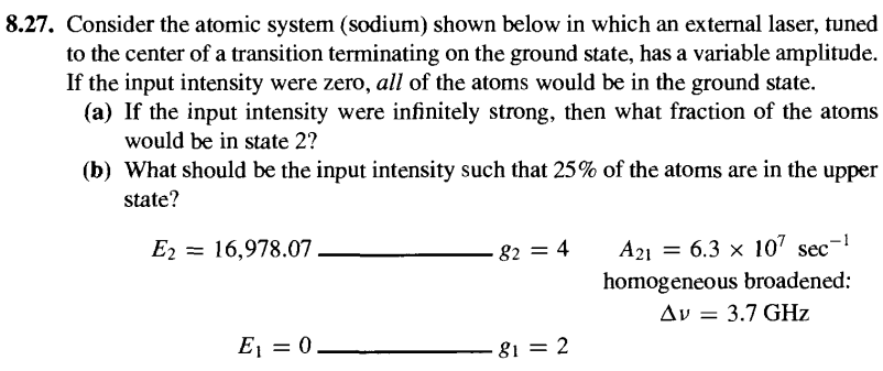
Solution:
(a)
$$I\rightarrow \infty \Rightarrow N_2-\frac{g_2}{g_1}N_1=0$$$$\frac{N_2}{N_2+N_1}=\frac{1}{1+\frac{g_1}{g_2}}=\frac{2}{3}$$(b)
$$\frac{N_2}{N_2+N_1}=\frac{1}{4} \Rightarrow N_1=3N_2$$$$\frac{dN_2}{dt}=-A_{21}N_2-\frac{\sigma I_{\nu}}{h\nu}[N_2-\frac{g_2}{g_1}N_1]=-A_{21}N_2-\frac{\sigma I_{\nu}}{h\nu}[N_2-(2)(3)N_2]=0$$$$-A_{21}+5\frac{\sigma I_{\nu}}{h\nu}=0$$$$I_{\nu} \approx 2.84 W/cm^2$$6.3 Homework 6
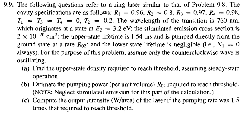
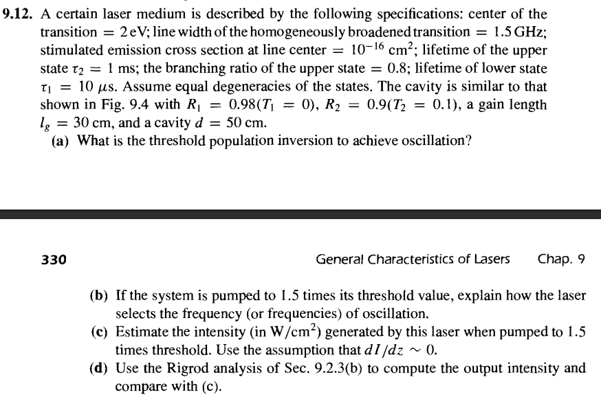
9.1, 9.5, 9.9, 9.12, 9.20
6.3.1 Problem 1
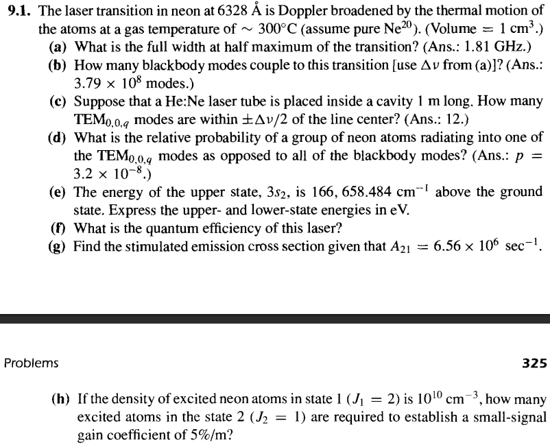
Solution:
(a)
$$\Delta\nu_D=(\frac{8kTln(2)}{Mc^2})^{1/2}\nu_0$$(b)
$$N_{BB}=\frac{8\pi n^3\nu^2}{c^3}V\cdot\Delta\nu$$(c)
$$N_L=\frac{\Delta\nu}{\Delta\nu_{FSR}}$$$$\Delta\nu_{FSR}=\frac{c}{2d}$$(d)
$$p=\frac{N_L}{N_{BB}}$$(e)
$$\bar{\nu}=\frac{1}{\lambda} \Rightarrow E=hc\bar{\nu}$$$$\Delta E=\frac{hc}{\lambda_{laser}}$$(f)
$$\eta_q=\frac{h\nu}{E_2}=\frac{\Delta E}{E_2}$$(g)
$$\sigma_{StE}=A_{21}\frac{\lambda^2}{8\pi n^2}g(\nu)$$$$g(\nu)=(\frac{4ln(2)}{\pi})^{1/2}\frac{1}{\Delta\nu_D}exp[-4ln(2)(\frac{\nu-\nu_0}{\Delta\nu_D})]$$(h)
$$\gamma_0(\nu)=\sigma_{StE}[N_2-\frac{g_2}{g_1}N_1]$$$$g_i=2J_i+1$$6.3.2 Problem 2
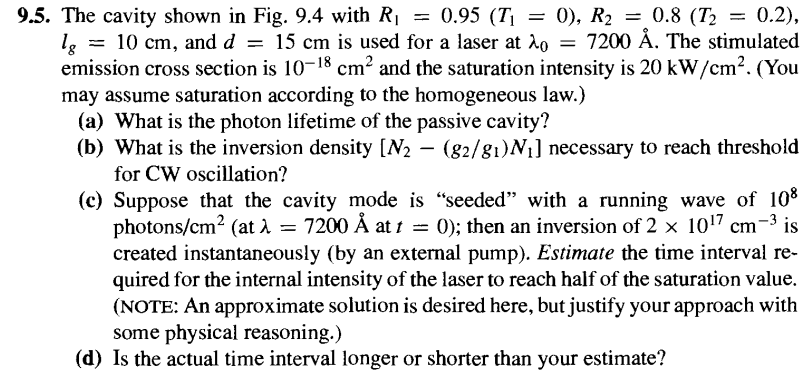
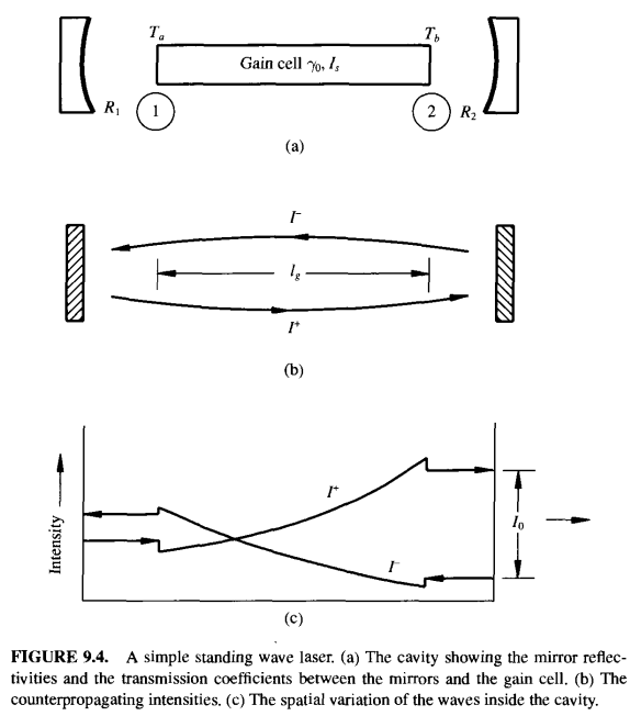
Solution:
(a)
$$\tau_p=\frac{2nd/c}{1-R_1R_2}$$(b)
Threshold condition:
$$R_1R_2e^{2\gamma_0 l_g}=1$$$$\gamma_0 = \sigma_{StE}N$$6.3.3 Problem 3
6.3.4 Problem 4
6.3.5 Problem 5

9.17: